
|
I. Ultra-High Precision Photometry
In these applications of ultra-high precision photometry, the desired
observed quantity is a change in magnitude; an accurate magnitude of
an object in the standard system is not required. This means that
ultra-high precision differential photometry is needed. The
need to find the difference in the brightnesses of two objects on a
frame make the task simpler; in this case, as long as the field is
relatively small, any changing transparency effects can be assumed to
be the same for all the objects. Ensemble averages make this
technique even more reliable. Given at least a few dozen stars in the
image, the assumption is made that the average magnitude of these
stars would remain constant from frame to frame, regardless of the
type or behavior of the individual stars. The ensemble average
provides a ``standard'' from which to measure the individual stars'
change in magnitude. These measurements will be used in a time series
analysis to search for stellar activity, which is essentially a
quasi-periodic phenomenon.
Even though the method of ensemble differential photometry is
well-suited to the task of detecting stellar activity, the
observations naturally suffer from noise, which makes the project a
challenge.
The trickier type of noise is 1/f noise, also called drift noise.
This type of noise appears small at high frequencies, but contains a
lot of power at low frequencies. An example of 1/f noise would be the
over all transparency of the atmosphere at an observing site. From
one night to the next, the general constituents in the atmosphere such
as particulate matter would be very similar. But over months or
years, the atmosphere at any site will change substantially, altering
the transparency.
II. Scientific Applications of Ultra-High Precision Photometry
III. CCD Photometry
IV. Current Status
V. Lessons Learned
VI. References
I. Ultra-High Precision Photometry
Observations of stellar activity on other solar-type stars could tell
us about the Sun's future behavior; the long-term changes in
brightness observed in other stars are very small, but even a small
change in the Sun's brightness could have a large impact on the
Earth's weather (Frohlich & Lean 1998). Fluctuations of ~2%
photometrically over a decade have been seen in local field stars
(Lockwood, Skiff & Radick 1997). Coherent oscillations in solar-type
stars also have very small amplitudes, but detecting them would let us
determine the interior structures of other stars. Finally, the
observation of transits due to planets around other stars would allow
us to constrain the properties of the planets more tightly than the
highly used doppler shift detection method. ``Ultra-high precision
photometry'' is necessary to study such small fluctuations in
brightness from astronomical objects.Types of Noise
Table 1 taken partially from Kjeldsen & Bedding (1998) lists some
typical noise sources. They can, broadly speaking, be divided into
two categories: white noise and 1/f noise. The fundamental source of
white noise is photon counting statistics. The noise is due to
intrinsic uncertainty in the rate at which photons arrive at the CCD;
this uncertainty goes as the square root of N if N is the number of
photons from the source. The uncertainty is a fundamental component
of the signal from the object and can never be eliminated; it can be
reduced by longer integration times to gather more photons (Kjeldsen
& Bedding 1998). For example, in order to achieve a precision of
0.1%, no fewer than one million photons must be received.
| Table 1: Noise Sources (From Kjeldsen & Bedding 1998) | ||
|---|---|---|
| Noise Source | Type of Noise | |
| Photons | Poisson statistics | white |
| Stellar | Granulation | non-white |
| Random light variation - drift | non-white | |
| Atmosphere | Scintillation | white |
| Transparency | non-white | |
| Extinction | non-white | |
| Refraction | non-white | |
| CCD | Sub-pixel structure | non-white |
| Large scale flat field structure | non-white | |
| Sensitivity stability | non-white | |
| Cosmic rays | white | |
| Charge transfer efficiency | non-white | |
| Dark current | white | |
| Read-out noise | white | |
| Gain | Variable temperature | non-white |
| Electronic drift | non-white | |
| Telescope | Stray light | non-white |
| Flexure | non-white |
Another difficulty with a time series analysis is that it is not possible to observe during the daylight hours. Consequently, during an observing run, equally-spaced gaps appear in the observations. Also, a typical observing run of several days to a week will have a gap of a few months until the next observing run. This periodic lack of information can affect the data's apparent periodicity, an effect known as aliasing. When analyzing the time series, not enough information may be available to find the fundamental period and so a longer period may be found instead, or an apparent period of roughly a day may be found.
The effects of aliasing are difficult to erase. Fortunately, since stellar activity timescales are on the order of months or years, the periodic diurnal gaps will not hinder us too badly. However, for shorter timescale variability, such as planetary transits and asteroseismology, the diurnal breaks must be eliminated through more or less continual observing. Gilliland et al. (1993) solved this problem by networking telescopes around the world for approximately one week of observations. Other solutions would be to observe from the South Pole during its winter (Heasley et al. 1996) or to observe via satellite (Kjeldsen & Bedding 1998).
II. Scientific Applications of Ultra-High Precision Photometry
Ultra-high precision photometry is a powerful technique which could be
applied to many scientific purposes. Low-level fluctuations occur in
several phenomena specifically related to stars.
The most easily detected transits would be by massive planets orbiting low mass stars. A Jupiter-size planet transiting a dM star will diminish the apparent brightness of the star ~0.02-0.08 magnitudes. However, an Earth-size planet's transit would be virtually indetectable from small-aperture, ground-based telescopes (Giampapa et al. 1995).
An advantage of detecting extra-solar planets by transits is that the amplitude of the transit is independent of the distance to the system. The drop in brightness observed during a transit can be distinguished from other forms of variability (such as stellar activity) in several ways: first, transits occur over just a few hours, while variability due to starspots would have a time scale comparable of days or longer; second, transits occur equally at all wavelengths, unlike variability due to stellar activity (Giampapa, et al. 1995); third, transits are strictly periodic, unlike variability due to starspots.
For Jupiter-size planets in orbits of less than 1AU around dM stars, the orbital periods would be 0.4-2.2 years. With these possible orbits, the transits would last 7.2-13.8 hours (Giampapa et al. 1995). One difficulty is that the time at which the transit will occur will not be known, so the candidates must be constantly monitored. Also, the planetary system may not be inclined favorably to our line of sight; a nearly edge-on system is required in order to observe the transit, which occurs for only about 1% of stars (Giampapa et al. 1995).
The Sun excites approximately 10^7 modes with amplitudes large enough for observation, even though the amplitudes of individual oscillation modes are very small: less than 10^(-6) relative displacement of the surface (Gilliland et al. 1993), or about 3 µ mag (Brown & Gilliland 1994). In frequency space, solar oscillations appear as nearly equally spaced peaks ranging from 2500-2800 µ Hz with a spacing of 68 µ Hz; an easily-distiguishable picket-fence pattern. (Gilliland et al. 1993).
The observed pulsations in the Sun are adiabatic pressure waves, the p-modes. The waves are likely excited by turbulence in the Sun's convection zone (Leibacher et al. 1985). In these modes, the interior pressure is the restoring force on the solar surface. (Brown & Gilliland 1994).
Solar-like stars would oscillate similarly to the Sun, but there are other types of pulsating stars, such as delta Scuti stars, roAp stars, and pulsating white dwarfs. In white dwarfs, the buoyancy of the stellar material acts as the restoring force; these modes of oscillations are called g-modes (Brown & Gilliland 1994). G-modes also exist in the Sun but are not observed due to their small surface amplitudes.
All oscillation modes in the Sun can be represented by classical spherical harmonics with orders described by n, l, and m. The radial order n corresponds to the number of vertical wavelengths in the oscillation, or alternatively the number of nodal lines along a radius of the Sun. The angular degree, l, of an oscillation is the number of surface nodal lines; consequently waves with a low value of l have very large wavelengths. The azimuthal order is m, which corresponds to the number of nodal lines that intersect the equator of the Sun; the absolute value of m must always be less than or equal to the angular degree l. A few special cases of oscillations exist. Purely radial oscillations have l=0. P-modes may be completely radial, but the ones generally observed are 5 <= l <= 100. G-modes must have l >= 1 (Leibacher et al. 1985, Brown & Gilliland 1994).
Stellar p-modes can be observed either in photometric intensity or in radial velocities. Upon reaching the top of the convective layer, the pressure waves ``jiggle'' the solar surface, which is observed as a doppler shift. The waves also alternately compress and rarify the stellar material, which causes temperature changes in the material, altering the observed intensity. Since the p-modes in the Sun originate in the convective layer, all stars with similar convection zones (later than approximately F5) should display p-modes. Stars with lower surface gravity and higher luminosity than the sun should pulsate with longer periods than the Sun does (Brown & Gilliland 1994); hotter and more evolved stars may have peak amplitudes of 20-50 µ mag and periods longer than the Sun's five minutes (Gilliland et al. 1993). Many of the modes that are distinguished in the Sun will average to zero over the stellar disk, so only modes with larger wavelengths (l=0,1,2,3) will be observable on other stars (Brown & Gilliland 1994, Leibacher et al. 1985).
To date, stellar oscillations have not been unambiguously detected in solar-like stars. Gilliland, et al., in 1993 conducted a campaign with a world-wide network of four-meter telescopes to search for oscillations in selected stars in M67; they reached a detection threshold of 20 µ mag, but did not find unambiguous evidence of oscillations.
More transitory activity consists of solar flares and prominences. Flares are eruptions of stellar material that occur in a few hours or less, originating from active sunspots. Prominences may be longer-lived. They consist of ionized gas that travels from the chromosphere along looping magnetic field lines and eventually falls back down to the chromosphere; they may extend far into the corona.
The majority of coronal activity consists of the structure of the corona itself. During times of low solar activity, the corona is featureless and generally isotropic. When the Sun is more active, however, the corona has gaps and streamers whose structure changes more quickly. Occasionally during periods of high solar activity, large amounts of material suddenly erupt from the corona and escape from the Sun; these are known as coronal mass ejections.
The solar cycle is a long-term cycling of solar activity, most obvious in the number of sunspots visible on the Sun at any point during the cycle. Approximately every eleven years, the number of sunspots reaches a maximum, declines to a minimum approximately 5.5 years later, and then increases again. The Sun's magnetic field switches polarity with each cycle. The Sun's total irradiance also varies on the same time scale.
The Sun is variable on a wide range of timescales: from a few minutes to the years that make up a solar cycle (Lockwood, Skiff, & Radick 1997, Pap et al. 1999). However, photospheric, chromospheric, and coronal effects related to the long-term solar cycle have similar timescales (Gilliland & Baliunas 1987).
The Sun's irradiance varies from three effects: the p-mode oscillations of the Sun, individual sunspots passing across the surface of the Sun and the 11-year solar cycle. Several experiments have been flown aboard spacecraft to measure the solar irradiance. The Solar Maximum Mission (SMM) found that when the cooler sunspots cross the Sun's surface, the Sun's brightness dims by as much as 0.2% (Lockwood, Skiff, & Radick 1997) or approximately 0.002 mag. The VIRGO experiment on the SOHO spacecraft showed that the amplitude of the variability caused by sunspots is larger at UV wavelengths than at red and IR wavelengths (Pap et al. 1999). This result is expected from thermal phenomena and will be expanded upon later.
The cause of the Sun's short-term variability is known to be related to sunspots. ACRIM data show that dips in the Sun's brightness are caused by the darker sunspots that move across the Sun's surface; the younger, more complex sunspot groups have a larger effect (Frohlich & Pap 1989). VIRGO data further show that the Sun's total irradiance is affected primarily by sunspots, but that the Sun's UV irradiance is more affected by plages associated with the sunspots (Pap et al. 1999). VIRGO also confrimed that active sunspot regions cause the strongest modulation in the brightness (Pap et al. 1999).
The solar cycle is much more difficult to monitor because of its long period. According to a composite record of the Sun's irradiance (from the HF, ACRIM I and II, ERBS, and VIRGO experiments), the Sun's irradiance was 0.1% (0.001 mag) higher during the sunspot maxima of 1980 and 1990 than during the minima of 1986 and 1996 (Frohlich & Lean 1998).
The variability of stars in a small number of open clusters has been studied to date, as well as the variability of some of the stars in the solar neighborhood:
Using spectroscopy of H-alpha and the Ca II infrared triplet, Soderblom, et al. (1993), determined v*sin(i) for many stars in the Pleiades. The values ranged from the detection threshold of 7 km/s to ~100 km/s. No specific correlation between rotation velocity and spectral type was seen, but the spread in rotation velocities appeared to have a pattern. Late-F and early-G dwarfs had a factor of five range in v*sin(i), while late-G and K dwarfs had a factor of twenty range. A small population of stars were called ultra fast rotators, with v*sin(i) >= 30 km/s.
The rotation periods that Radick, et al. (1987), found ranged from approximately five days to thirteen days; the periods tended to increase with spectral type. A typical G star in the Hyades rotates three to four times faster than the Sun. Through the Ca II H and K line observations, they determined that drops in photometric brightness correspond to increases in the H and K flux, which suggests that starspots and plages coincide on the stars' surfaces.
Stauffer, et al. (1991), observed the H-alpha line on low-mass Hyades stars, since H-alpha equivalent widths also indicate the amount of chromospheric activity present on a star. Comparing their data to that from the Hyades and field M dwarfs, they concluded that chromospheric activity decreases with the age of the star. They also observed that H-alpha emission or absorption equivalent widths may vary with plages on the star in a manner similar to the solar cycle.
Sun-like field stars in the solar neighborhood have also been studied to learn about their stellar activity. Lockwood, Skiff, & Radick (1997) reported on ten years of observations of nearby sun-like stars in Stromgren b and y. They observed forty-one stars, approximately three-quarters of them from the Mt. Wilson HK Program. They discovered that late-F through M stars had rotational variability ranging from ~0.003 mag to ~0.05 mag. The yearly variability was approximately 0.015 mag (See Table 2.). They possibly uncovered ``solar cycle'' decade-scale variations of 0.03 mag peak-to-peak, but could not find any periods. In their study, the amplitude of the yearly variability was correlated with (B-V) color.
Radick, et al. (1998), combined their photometric measurements (Lockwood, Skiff, & Radick 1997) with the results from the Mt. Wilson HK Project for the thirty-four stars included in both programs. They found that the long-term activity of the nearby stars was roughly segregated by mass: those stars more massive than the Sun had low-amplitude cycles, but those stars less massive than the Sun tended to have high-amplitude cycles. Also, they observed that young, active stars tend to become fainter as their chromospheric emission increases, but older stars, including the Sun, tend to becoming brighter as their chromospheric emission increases. This could be the cause of variability for each star: younger stars decrease in brightness because starspots are the greatest influence, but for older stars, the dominant plages cause an increase in brightness. They determined that both long-term and short-term (rotational) variability was correlated to the over all level of chromospheric activity of the star.
The ``Sun in Time'' project, which is a multi-wavelength study of nearby, solar-type stars, was begun in 1988 by Bochanski, et al. (2000). Preliminary photometric results for rotational variability for these stars has been released; the youngest stars, ~70 Myr (O'Dell et al. 1995), have variations of 0.03-0.09 mag, while the stars older than ~2 Gyr have variations less than 0.01 mag. These results are included below in Table 2.
The primary difficulty in observing field stars is determining their ages, which is also a problem with the Mt. Wilson HK Project. The estimated ages of stars in the project come from indirect techniques. The abundances of certain elements such as lithium compared to abundances expected from stellar models can allow an approximate age determination, keeping in mind that metal-poor stars are not necessarily older than metal-rich stars (Friel & Janes 1993). Another method is to measure the rotational velocity of the star spectroscopically; younger stars are assumed to have shorter rotation periods. The amount of chromospheric emission is another test: younger stars are expected to be more chromospherically active. However, the reasoning in some of these methods is rather circular. A star deemed young because of its high chromospheric activity or rotational velocity can not then be used to show that young stars possess these properties. This is a fundamental problem not easily overcome.
We have chosen to search for stellar variability in open clusters since we know their ages. The first task is to observe the clusters and perform photometry upon the images. Figure A, which shows graphically the results in Table 2, also demonstrates that the precision of our observations is approaching that needed to observe these low-level variations.
| Table 2: Photometric Variability | ||||
|---|---|---|---|---|
| Rotational (Days) | ||||
| Spectral Type | Amp. (mag) | Target | Age | Reference |
| G | ~0.035 | IC 2602 | 35 Myr | Barnes et al. 1999 |
| K | ~0.033 | IC 2602 | 35 Myr | Barnes et al. 1999 |
| M | ~0.041 | IC 2602 | 35 Myr | Barnes et al. 1999 |
| G | ~0.095 | Pleiades | 70 Myr | Krishnamurthi et al. 1998 |
| K | ~0.096 | Pleiades | 70 Myr | Krishnamurthi et al. 1998 |
| M | ~0.06 | Pleiades | 70 Myr | Krishnamurthi et al. 1998 |
| G | ~0.03 - 0.09 | local dwarfs | ~70 Myr | Bochanski et al. 2000 |
| G | ~0.0078 | Coma | 430 Myr | Radick, Skiff, & Lockwood 1990 |
| late-F | ~0.032 | Hyades | 700 Myr | Radick et al. 1987 |
| G | ~0.040 | Hyades | 700 Myr | Radick et al. 1987 |
| K | ~0.040 | Hyades | 700 Myr | Radick et al. 1987 |
| F | ~0.0027 | HK Project | ? | Lockwood, Skiff, & Radick 1997 |
| G | ~0.0038 | HK Project | ? | Lockwood, Skiff, & Radick 1997 |
| K | ~0.0053 | HK Project | ? | Lockwood, Skiff, & Radick 1997 |
| M | ~0.08 | HK Project | ? | Lockwood, Skiff, & Radick 1997 |
| G | < 0.01 | local dwarfs | ~2 Gyr | Bochanski et al. 2000 |
| G | 0.002 | Sun | 4.6 Gyr | Lockwood, Skiff, & Radick 1997 |
| Long-Term (Years) | ||||
| Spectral Type | Amp. (mag) | Target | Age | Reference |
| G | ~0.015 | Coma | 430 Myr | Radick, Skiff, & Lockwood 1990 |
| G | ~0.015 | Hyades | 700 Myr | Radick et al. 1987 |
| F | ~0.0028 | HK Project | ? | Lockwood, Skiff, & Radick 1997 |
| G | ~0.0193 | HK Project | ? | Lockwood, Skiff, & Radick 1997 |
| K | ~0.0118 | HK Project | ? | Lockwood, Skiff, & Radick 1997 |
| G | 0.001 | Sun | 4.6 Gyr | Frohlich & Lean 1998 |
A bias frame is an image taken with zero exposure time (with the shutter closed). Consequently, it is also a measure of the zero point of the CCD electronics. Once the overscan information is applied to the bias frame, the level of the bias frame would be zero if the CCD were perfect. Unfortunately, this is never the case. Once the overscan is applied, the bias frame may show a low-level pattern. This frame may be subtracted from any object frame in order to remove this pattern.
The dark level of a CCD is signal that accumulates during an integration with the shutter closed; the signal is due to thermal noise. There may also be ``hot pixels'' on the CCD that develop unusually large amounts of charge. Some pixels may even be LEDs which generate their own light. Typically a few dark frames of various lengths are taken; if the dark levels are non-negligible, an average dark frame may be scaled to the integration time of an object frame, and then subtracted from the object frame.
The deferred charge correction is applied to correct for nonlinearities of the CCD at low levels of intensity. In essence, during readout, not every pixel on the CCD may ``pass on'' its photons completely. We have neglected this effect.
The IRAF program and various applications in the base IRAF package as well as the noao.imred.ccdred package are utilized. Initially, at least, each night of observations is processed separately with its own calibration images. The routine ccdproc is used to apply the overscan and to trim the bias images to the correct size. Then the images are averaged using the imcombine routine. The dark images are calibrated with ccdproc which applies the overscan, trimming, and averaged bias image as a zero correction. The dark images are then averaged with imcombine. Finally, this initial step is completed when the object and flat field images are calibrated with ccdproc which applies the overscan, trimming, zero correction, and dark correction. A dark correction was not always applied, as its value generally was negligible.
A shutter correction for the SITe CCD can be created by comparing long integration flats to short integration flats. A long integration flat should be twenty seconds or longer. As many of these flats as is practical are averaged into one flat: the Long Flat. This is done with the routine imcombine.
All flats that are two seconds or shorter are flatted with the Long Flat. This is done with the ccdproc routine and choosing a flat fielding correction; however, the short flats have to have their image types changed with IRAF's routine hedit to ``object'' from ``flat'' so the routine will work. The resulting images clearly show the closing shutter. These will be designated the Interim Images; five or six Interim Images are sufficient.
In order to use these Interim Images to create a shutter correction, the number of ADUs in the center of the Image is to be found. Using the IRAF routine implot, the central part of the image can be easily examined. The integration time of the center pixel is the true integration time, so the number of photons gathered in this pixel is used to normalize the correction image. A shutter correction image can then be made from each of the Interim Images with the following recipe (image variables are indicated with an accent):
S' = (M-I')/(M) * T,
where M is the number of ADUs in the center of the Interim Image,
I' is the Interim Image, and T is the exposure time of
the short flat that was made into the Interim Image. S' is then the
shutter correction. This formula scales the ``picture'' of the
shutter according to both the intensity of the Interim Image and the
exposure time of the Interim Image. Image arithmetic may be done with
the IRAF routine imarith.
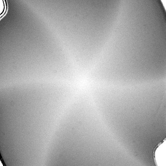
Once a shutter correction has been made from each of the Interim Images, all of the shutter correction images are averaged to make a master shutter correction, again using imcombine. This master shutter correction (Figure B) is tested on a few of the (unflatted) short flats to see if it is effective. Some brief testing has demonstrated that the master shutter correction is independent of filter. It also does not seem to change over time, at least on time scales of a few months. However, it is recommended that a master shutter correction image be made for each observing run. On a typical shutter correction image, which is representative of a one-second exposure, the number of ADUs received at the edge of the CCD is only 1.8% of that received at the center.
Once the master shutter correction has been made, each image can be corrected with the following formula:
I'[true] (1 - S'/T) = I'[obs],
which can be rearranged as:
I'[true] =I'[obs]/(T - S'*T).
In this case, S' is the master shutter correction image,
I'[obs] is the observed image, and I'[true] is the
corrected image. A longer image will obviously be less affected by
the slow shutter, and so longer images have a smaller correction.
Once the master shutter correction image is made, correcting the individual images of the run is very routine. An IRAF procedure has been written which may be used to correct lists of images. The flat field images as well as the object images are corrected for the shutter pattern.
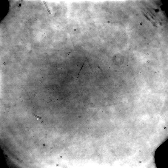
The flat fields have previously been calibrated for overscan, trimming, bias, dark levels, and the shutter pattern. Now all of the flat fields for each filter are averaged into a ``master'' flat field for that filter using the routine imcombine. The result is that each night has a ``master'' flat field in each of the filters that was used for observations. A Perkins flat field can be seen in Figure C.
The ``master'' flat fields for the same filter on different nights should be compared. If they have no major differences (new dust rings, for example), then the ``master'' flat fields for a filter may be averaged into one flat with imcombine. However, if the flats differ significantly, then each night's flat should be used to calibrate only that night's observations. Once the final flat field for each filter has been created, the object images are corrected by the appropriate flat field using ccdproc. However, it appears that this standard type of flat field correction may be inadequate, as will be discussed later. Flat fields are another source of 1/f noise: the flat fields taken on successive nights will be very similar, but after weeks or months, they will be substantially different. The sensitivity of the CCD pixels may gradually change over time, the spectrum of the twilight sky observed will be different, and the ubiquitous dust seen in flat fields may have changed.
In aperture photometry, an aperture of a certain radius is placed around the star and the intensity (in ADUs) within the aperture is summed. In order to account for the sky background, an annulus is extended around the aperture and the intensity within it is summed. Then the difference in the two values is the intensity from only the star. The resulting intensity is scaled according to the exposure time of the image and then converted into an instrumental magnitude according to the usual logarithmic formula.
PSF-fitting photometry is more complex. A functional form for the expected PSF of the star is determined prior to analysis. A number of reasonably bright, but unsaturated stars are chosen to be fit to this function. This fit may also included a zero level that would correspond to the sky background. The resulting fit is saved as the PSF for that frame. Subsequently, all stars in the frame are fit to the saved PSF; the ``height'' in ADUs of the PSF fit to the star corresponds to the star's intensity, analogous to the aperture photometry method. Again, scaling the intensity for the exposure time, the magnitude of the star can be derived.
In general, aperture photometry is sufficient for bright stars, since their signal dominates the sky and other CCD noise. PSF-fitting becomes more precise as the stars become fainter and harder to distinguish from the background noise.
The Stellar Photometry Software (SPS, Janes & Heasley 1993) program performs both aperture and PSF-fitting photometry on all stars on every image. Fortunately, SPS is programmed for a ``batch'' processing mode, where it is given lists of images and reduction commands and can perform the photometry on all the images without user interaction.
Several parameters of the CCD must be specified. Other parameters must be determined through interactive use of SPS on some typical images. In order to locate the stars on the image, SPS must be told the typical stellar FWHM for the observations. For the aperture photometry, the aperture size and sky annulus must be specified. Since SPS does PSF-fitting photometry, an appropriate diameter for the PSF must be determined. In the PSF creation process, SPS must have a tolerance level for choosing proper stars to make the PSF. All of these parameters were experimented with to optimize the performance of SPS. Fortunately, the parameters vary little from night to night or even observing run to observing run, for the same CCD. SPS will also use each the appropriate input parameters and its own measurements to predict an error for each magnitude measurement. The parameters for the SITe CCD are:
| Table 3: Observing Runs (Processed) | ||
|---|---|---|
| Telescope | No. of Nights | No. of Frames |
| Mt. Laguna Observatory | 41 | 878 |
| Perkins Telescope | 18 | 992 |
Star 1017 is a previously known delta Scuti star, with a period of 0.078587 days. It has an apparent V magnitude of 15.53 and was observed at the Mt. Laguna Observatory from August 1996 to November 1998. Secondary oscillation periods of the star could be contributing to scatter within the plot. (Figure D.)
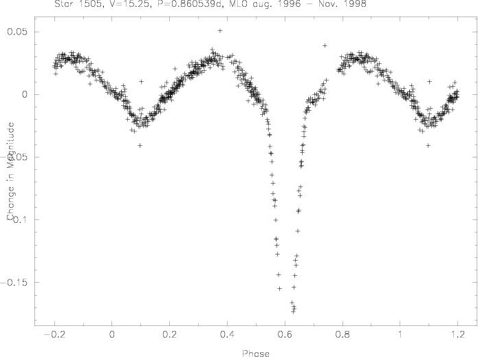
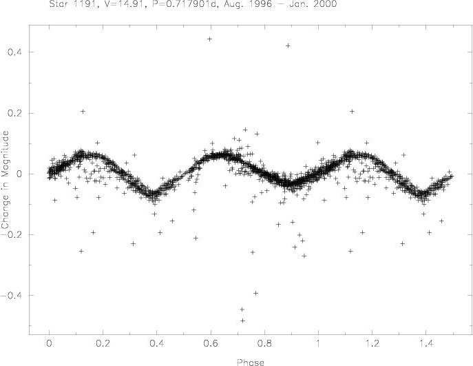
Star 1505 is a previously known eclipsing binary star. It has a V magnitude of 15.25 and a period of 0.860539d. It was observed on the Mt. Laguna Observatory telescope from August 1996 to November 1998. (Figure E.) An eclipsing binary that was discovered using the Perkins Telescope is star 1191. It has a V magnitude of 14.91 and a period of 0.717901d. Once it was discovered in the Perkins Telescope data, a check of Mt. Laguna Observatory data revealed that it was observed there as well, so it has been observed from August 1996 to January 2000. (Figure F.)
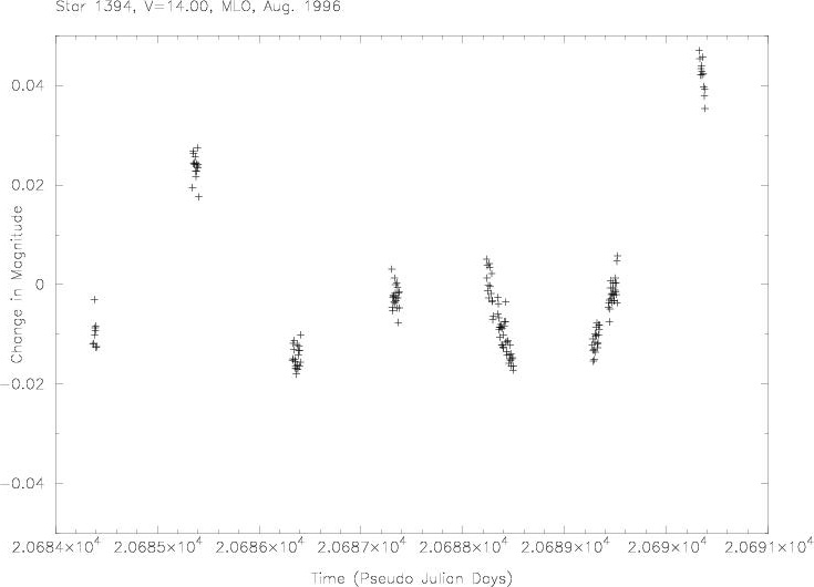
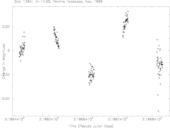
We have also found a number of stars with unexplained variations in our data. A few stars clearly seem to be showing erratic variation, but we cannot find single periods for them. One such star is 1394, V=14.00. This star apparently varies significantly more than the errors in the measurements in each observing run. The variations are visible in the Mt. Laguna Observatory run of August 1996 and in the Perkins Telescope run of November 1999. (Figures G & H.)
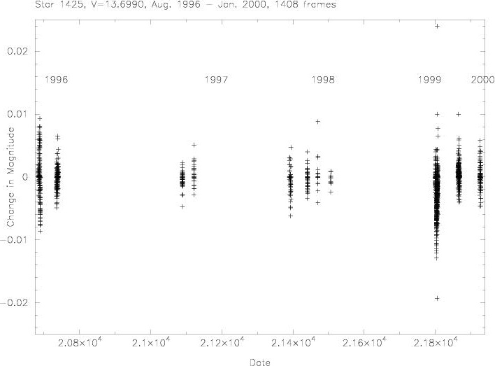
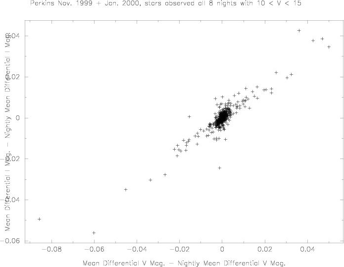
To illustrate the precision of our data so far, the measurements of the changes in magnitude of a bright star in NGC 7789 have been plotted in Figure I. Each vertical scattering of measurements constitutes an observing run, from August 1996 to January 2000. The plot shows that the precision of the measurements has been consistent over these three years, but also that the Mt. Laguna Observatory data and the Perkins Telescope data match well.
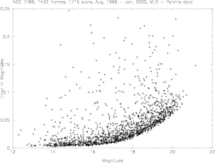
To give a broader view of our overall precision, the magnitude of the stars of NGC 7789 versus the error in the magnitudes (over the time series) has been plotted in Figure J. These data span from August 1996 on the Mt. Laguna Telescope to January 2000 on the Perkins Telescope. The plot shows the measurements of 1715 stars from 1432 images. A substantial portion of the stars have errors less than 0.01 magnitudes. The ``lower limit'' curve on the graph is approximately twice what would be expected strictly from Poisson statistics. This precision is still not good enough to confidently detect stellar activity. However, the data are precise enough for excellent color-magnitude diagrams and standard UBV photometry, which fall under the purview of other members of our group.
| Table 4: Typical V and I Error | |||||
|---|---|---|---|---|---|
| V Star | m(v) | V Error | I Star | m(i) | I Error |
| 353 | 15.7001 | 0.0189 | 94 | 15.7565 | 0.0272 |
| 377 | 15.6315 | 0.0196 | 58 | 15.8451 | 0.0472 |
| 706 | 15.7197 | 0.1201 | 58 | 15.7991 | 0.0337 |
| 715 | 15.6039 | 0.0186 | 59 | 15.7461 | 0.0255 |
| Table 5 | |||||
|---|---|---|---|---|---|
| Brighter V Star | Fainter V Star | ||||
| Star | m(v) | Error | Star | m(v) | Error |
| 63 | 10.6729 | 0.0009 | 39 | 17.6372 | 0.1015 |
| 123 | 10.7126 | 0.0009 | 77 | 17.4658 | 0.0857 |
| 143 | 10.7429 | 0.0009 | 282 | 17.5409 | 0.0921 |
| 155 | 10.7667 | 0.0009 | 327 | 17.4656 | 0.0852 |
The large quantity of dome flats for each telescope allowed us to
assess the performance of each CCD. In order to determine the true
nature of the noise in the dome flats (and thus the CCDs), we had to
isolate the noise. All the dome flats for each evening were averaged.
A smoothed version of this average dome flat was subtracted from
itself to remove the large scale features. Then two nights were
compared to each other by subtracting one from the other. The
resulting image was trimmed to eliminate edge effects.
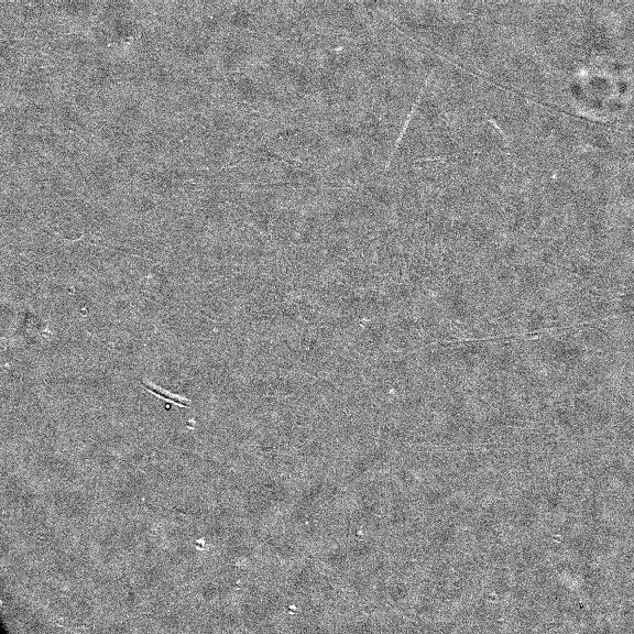
When this was done with V dome flats taken on the Perkins with the
SITe CCD on 9/12/99 and 9/14/99, the resulting image can be seen in Figure K. The image has the
following statistics:
V. Lessons Learned
Comparing the data from the Mt. Laguna Observatory and the Perkins
Telescope has allowed us to identify some of our nagging noise
sources. Inadequate flat fielding seems to be the most difficult
problem to solve.Flat Fielding Experiments
We have analyzed flat fields from both the MLO and Perkins telescopes
in an effort to determine how effective they are.Mt. Laguna Observatory and Perkins Telescope, September 1999
In September 1999, we attempted to use the Perkins Telescope (with
SITe CCD), Hall Telescope (with Navy CCD), and MLO 1m telescope (with
Loral CCD) simultaneously. If successful, concurrent measurements
would have provided a way to check if the fluctuations in each star
were due to instrumental or environmental conditions, or if they were
intrinsic to the star; a truly varying star would be observed to vary
from all of the telescopes. Unfortunately, due to the weather, only
one night of simultaneous observations was possible and even then the
conditions in Flagstaff were not ideal. Regardless of the weather,
100 dome flats were taken through the V filter on several days at each
telescope for later analysis.
When the previous analysis was done with V dome flats taken on the
Hall telescope with the Navy CCD for 9/11/99 and 9/12/99, the
resulting image had the following statistics:
The same analysis was done with V dome flats taken on the MLO 1m
telescope on 9/12/99 and 9/13/99. The resulting image (Figure L) had the
following statistics:
As an example, here are some statistics for the V dome flats from 11/11/99 subtracted from the V dome flats from 11/15/99, which were the first and last nights of the observing run:
Also for the I dome flats (Figure N) for the same nights:
In a similar analysis, the master dome flats in V for each night were averaged together to make a ``total'' V dome flat. A smoothed version of this total flat was subtracted from itself. The same procedure was done for the V sky flats, the I dome flats, and the I sky flats. Then, the resulting V sky flat (with the large-scale structure removed) was subtracted from the total V dome flat. The same was done with the I total sky flat and dome flat. The resulting two images (trimmed for edge effects) should show the small-scale differences between the dome and sky flats in each filter.
The V result can be seen in Figure Q. The V statistics:
This type of color index analysis has been helpful, and in Figure S, the behavior is roughly seen. Unfortunately, our measured I magnitudes have inexplicably higher errors in general, despite the same photon count level as in the V filter. This strategy has not yielded improved results as yet.
The Perkins telescope is an improvement over the MLO 1m telescope simply because of the Perkins' larger aperture. Higher photon counts will reduce the photon noise considerably. Also, a new filter set might be advantageous in this respect. With two filters that range from 4000-6000 angstroms and 5000-7000 angstroms we would gather more photons, and yet the fluctuations in brightness through each filter should be highly correlated.
The completion of PRISM will allow the possibility of spectrophotometry. The zero order spectrum would not be dispersed and would be a measure of the total brightness (through a filter) of the star. The first order spectrum would be dispersed to one side of the CCD where various spectral lines could be monitored or variations in brightness of the red end of the spectrum compared to the blue end could be determined. In this way, we could obtain our color fluctuation ``double-check'' and total intensity measurement simultaneously. An additional check that the intensity in the first order and higher order are equal would also provide information on the stability of the CCD. Also, longer exposure times would be possible since the light from a star is dispersed, allowing more photons to be gathered.
Obviously not all of the stars in the cluster would be able to be observed; an aperture mask allowing observations dozens of specific stars would be needed. The aperture mask would also ensure that each time the star cluster is observed the same stars will be placed on the same pixels of the CCD. Consequently, comparing the stars to themselves on each frame will compensate for any flat fielding or pixel irregularities. Since each pixel in the spectrum will always be receiving the same wavelengths of photons, it can be calibrated for those specific wavelengths so that differing spectral sensitivities between pixels will not be a problem.