Very Wide Binaries and Other Comoving Stellar Companions: A Bayesian Analysis of the Hipparcos Catalogue
Abstract.
We develop Bayesian statistical methods for discovering and assigning probabilities to non-random (e.g., physical) stellar companions. These companions are either presently bound or were previously bound. The probabilities depend on similarities in corrected proper motion parallel and perpendicular to the brighter component's motion, parallax, and the local phase-space density of field stars. Control experiments are conducted to understand the behavior of false positives. The technique is applied to the Hipparcos Catalogue within 100 pc. This is the first all-sky survey to locate escaped companions still drifting along with each other. In the <100 pc distance range, ≈220 high probability companions with separations between 0.01 – 1 pc are found. The first evidence for a population (≈300) of companions separated by 1 – 8 pc is found. We find these previously unnoticed naked-eye companions (both with V<6th mag): Capella & 50 Per, δ Vel & HIP 43797, Alioth (ε UMa), Megrez (δ UMa) & Alcor (80 UMA), γ & τ Cen, φ Eri & η Hor, 62 & 63 Cnc, γ & τ Per, ζ & δ Hya, β01, β02 & β03 Tuc, N Vel & HIP 47479, HIP 98174 & HIP 97646, 44 & 58 Oph, s Eri & HIP 14913, and π & ρ Cep. High probability fainter companions > 6th mag) of primaries with V<4th mag are found for: Fomalhaut (α PsA), γ UMa, α Lib, Alvahet (ι Cephi), δ Ara, β Ser, ι Peg, β Pic, κ Phe and γ Tuc.
Table of Contents
§ 1. Introduction
The observed binarity and multiplicity rates of stars are significant
clues to star formation processes and galactic dynamics. For example,
the mass-ratio distribution among pre-main-sequence binaries1
After formation, the evolution of binaries is determined by dynamical processes. In high to moderate density environments, most pairs with separations of a few hundred to a few thousand AU are broken up within a few million years (Parker et al., 2009). Outside of these high density regions, Galactic tides and weak interactions with passing stars peel off stars with separations of a few times 10,000 AU on a time scale of about 10 Gyr ((Heggie, 1975; Weinberg et al., 1987)).
Until quite recently, stars were commonly assumed to quickly leave the scene once they become unbound. However, recent simulations find that escaping stars drift apart with relative velocity ≈ 1 km s-1 and remain within a few 100 pc of the primary for billions of years (Jiang & Tremaine, 2010). In these simulations the large scale potential is dominated by Galactic tides, while local perturbations to the large-scale potential are dominated by stars. Their model does not include molecular clouds, spiral arms, or dark-matter subhalos. The simulations indicate that the binarity rate decreases with separation out until several tidal radii, at which point the rate actually increases and peaks at 100 – 200 pc. In addition, since the Galactic gravity field dominates the trajectories of escaped stars, they travel along with their ex-primaries, trailing or leading at roughly constant Galactic radii (like a tidal stream, but of only two or three stars).
On the other hand, if, locally, there are many dark matter subhalos, companions would be more quickly torn away and evidence of previous binaries would be lost. Thus, observational determination of the frequency and ages of escaped companions in similar orbits should tell us much about the small scale structure of the Galactic gravity field, the Oort A- and B-constants, and place stringent constraints on dark matter subhalos.
Existing double star catalogs, such as the WDS (Mason et al., 2001), are
mostly populated with systems selected using fairly simple criteria
such as proximity in the plane of the sky or common proper motions
(CPM) of high proper motion stars. Very often, pairs await
confirmation of orbital motions before being accepted as a physical
pair which, obviously, selects against wide binaries.
In a work based on double stars extracted from a large number of catalogs,
one of us found that the apparent binarity rate changes dramatically
both with distance from the Sun, and with apparent magnitude
(Olling, 2005a).
In that work many catalogs2
§ 1.1. Why Very Wide Binaries?
Parker et al. (2009) indicate that “hard binaries” with semi-major axis a ≤ 50 AU are almost never affected by dynamical processes in either the field or inside clusters, while “intermediate binaries” (50 ≤ a ≤ 1,000) can be highly affected by dynamical processes, especially if they are formed in dense star clusters. Unevolved “wide binaries” with a > 1,000 AU can only have formed in low density starforming regions with densities less than a few stars per pc3, the so-called “isolated star formation” mode (Goodwin, 2010). However, of order 15% of G-type dwarfs are found in wide binary systems, with a ≥ 104 AU, which even exceeds the size of isolated star formation regions. It is thought that systems of this size can only form during the dissolution phase of low density clusters (Kouwenhoven et al., 2010).
From a Galactic dynamics perspective, one can expect binary stars with
separation up to about the tidal or Jacobi radius,
rJ,
while their relative velocities should be
about the Jacobi velocity (![]() ):
):
 |
(1) | ||
 |
(2) |
(Jiang & Tremaine, 2010), where ![]() , is the gravitational constant,
Ω the angular velocity of the Galaxy at the Solar circle,
A
is Oort's A constant, and M1 and M2 are the masses of the
components.
The value of 1.7 pc is valid for the canonical values for
the Galactic constants and individual masses of 1
, is the gravitational constant,
Ω the angular velocity of the Galaxy at the Solar circle,
A
is Oort's A constant, and M1 and M2 are the masses of the
components.
The value of 1.7 pc is valid for the canonical values for
the Galactic constants and individual masses of 1 ![]() . Note that the
tidal radius depends weakly, only as the cube root, of total mass.
Thus, if it is the case
that systems that become unbound remain “close companions” for a very
long time, then the region where bound or almost bound systems can be
found would extend much farther than has been previously suggested
[0.1 – 0.2 pc; e.g., Heggie (1975); Bahcall & Soneira (1981); Retterer & King (1982); Weinberg et al. (1987); Quinn et al. (2009)].
This all suggests that separations from 10,000 AU to several parsecs is in
need of much further study.
. Note that the
tidal radius depends weakly, only as the cube root, of total mass.
Thus, if it is the case
that systems that become unbound remain “close companions” for a very
long time, then the region where bound or almost bound systems can be
found would extend much farther than has been previously suggested
[0.1 – 0.2 pc; e.g., Heggie (1975); Bahcall & Soneira (1981); Retterer & King (1982); Weinberg et al. (1987); Quinn et al. (2009)].
This all suggests that separations from 10,000 AU to several parsecs is in
need of much further study.
§ 1.2. Some Previous Searches for Very Wide Binaries
The search for companions of high proper motion pairs in
astrometric catalogs is ongoing; e.g., Levine (2005) use the
USNO-B1 catalog (Monet et al., 2003), Gould & Kollmeier (2004) use the USNO-B1 and
2MASS (Skrutski et al., 2006), Makarov et al. (2008) use the
NOMAD3![]() 65 in the WDS, while the latter work focuses on
the α Lib + KU Lib system with a separation of 2
65 in the WDS, while the latter work focuses on
the α Lib + KU Lib system with a separation of 2![]() 6 (1.05 pc).
In these works, the focus has been on common proper motions.
However, to search for the widest bound systems and for recently escaped
companions, one must look at separations >1 pc,
which corresponds to several degrees of separations for stars within 100 pc.
But, projection effects cause companions with similar space velocities to
have dissimilar proper motion and radial velocities, hence at very
wide separations, common
proper motion studies will miss true companions and may even lead to misidentifications.
In §§3.2, we describe how to take these geometric effects into account.
6 (1.05 pc).
In these works, the focus has been on common proper motions.
However, to search for the widest bound systems and for recently escaped
companions, one must look at separations >1 pc,
which corresponds to several degrees of separations for stars within 100 pc.
But, projection effects cause companions with similar space velocities to
have dissimilar proper motion and radial velocities, hence at very
wide separations, common
proper motion studies will miss true companions and may even lead to misidentifications.
In §§3.2, we describe how to take these geometric effects into account.
Finding companions of nearby stars by rigorous statistical analyses is a fast way to discover additional nearby stars. It may also be a means of discovering more nearby brown dwarfs and white dwarfs, provided many faint candidate stars are included, as in the larger Tycho-2 (TY2) or UCAC3 catalogs. Finally, the discovery of a substantial number of late-type stars that are paired to higher mass stars can help significantly in establishing the metallicity and temperature scales for these low-mass systems (presumably, both components have the same [Fe/H]).
Therefore, it would be fruitful to attempt to construct a statistically robust catalog of astrometric companions (both bound systems and escaped binary components) with well defined selection criteria by datamining modern astrometric catalogs. The astrometric catalogs such as HIP, TY2, UCAC3 and NOMAD provide order of magnitude better proper motions than previous catalogs [but see the cautionary notes by Makarov et al. (2008) on possible systematic errors for faint NOMAD sources]. In this paper, a methodology based on Bayesian statistics is discussed and applied to the stars in just the HIP that are within 100 pc. In a future work, we will present results of applying these techniques to stars in the TY2 that may be companions to stars in HIP.
Throughout this paper, we use “d ” for distance (in pc),
“ ” for 3-d radial separation,
“
” for 3-d radial separation,
“ ” for parallax, “
 ” for proper motion,
“
” for proper motion,
“ ” for angular separation, and “
 ” for semi-major
axis, unless otherwise stated. The sub- and superscripts “
” for semi-major
axis, unless otherwise stated. The sub- and superscripts “ ,” “
,” “ ,”
and “
,”
and “ ” are used to refer to properties of
primaries, companion candidates and stars in “the field,”
respectively.
” are used to refer to properties of
primaries, companion candidates and stars in “the field,”
respectively.
§ 2. Multiplicity: Recent Developments
In their study, Duquennoy & Mayor (1991) (hereafter DM91) use their radial velocity data in combination with existing astrometric binaries to determine the distribution of periods of main-sequence G stars within 22 pc. They find that the parent distribution function (PDF) of periods is approximately Gaussian in the logarithm of the period,
 |
 |
 |
(3) | ||
where ![]() is the period in days.
The peak is at
is the period in days.
The peak is at ![]() years (≈ 35 AU), while
the 1-σ boundaries are 316 days (≈ 1 AU)
and 34,000 years (≈ 1,212 AU).
From their data, DM91 estimate a binary fraction of ≈67%.
DM91 also find that their observations are consistent with the assumption
that secondaries are drawn randomly from the initial mass function
(IMF) below the primary; therefore, companions are usually considerably fainter
than the primary.
There is debate in the
literature over the exact shape of the PDF: DM91's Gaussian
shape was first proposed by Kuiper (1942) versus Öpik
classical power-law distribution (Öpik, 1924). Because the integral
of the Öpik-power-law distribution diverges it must break
down. This is indeed observed at small and large separation (e.g., Goldberg et al. (2003); Chanamé & Gould (2004); Lépine & Bongiorno (2006), and references therein).
years (≈ 35 AU), while
the 1-σ boundaries are 316 days (≈ 1 AU)
and 34,000 years (≈ 1,212 AU).
From their data, DM91 estimate a binary fraction of ≈67%.
DM91 also find that their observations are consistent with the assumption
that secondaries are drawn randomly from the initial mass function
(IMF) below the primary; therefore, companions are usually considerably fainter
than the primary.
There is debate in the
literature over the exact shape of the PDF: DM91's Gaussian
shape was first proposed by Kuiper (1942) versus Öpik
classical power-law distribution (Öpik, 1924). Because the integral
of the Öpik-power-law distribution diverges it must break
down. This is indeed observed at small and large separation (e.g., Goldberg et al. (2003); Chanamé & Gould (2004); Lépine & Bongiorno (2006), and references therein).
Raghavan (2009), in his dissertation, presents an impressive body of work on a sample of stars that significantly extends the DM91 sample. He scrutinized 454 Sun-like stars within 25 pc by pulling together up-to-date radial velocity surveys and the best Hipparcos astrometry, while he also performed a large survey with the CHARA interferometer for close-in binaries. Following in the footsteps of recent wide-binary searches, he “blinked” between early- and late-epoch sky-survey images, out to radii of about 10′, or 10 kAU. He concludes that (55 ± 3)% of stellar systems are single stars. For the 25 pc sample, we search for companions with separations up to 120 times larger than those blinked by Raghavan (2009).
§ 3. Methodology
Although astronomers have been searching for and finding physically associated pairs of stars since the time of Galileo, there have not been thorough studies to explicitly assign probabilities of association. In this pilot project, we search for common proper-motion stellar multiples out to very large separations, as far as is practical, and set probabilities for these to be more than merely coincidental. We do not limit ourselves necessarily to high proper-motion pairs as has been done in the past (Gould & Chanamé, 2004; Lépine & Bongiorno, 2006): although stars with field stellar density exceeding some threshold in a 5 dimensional box given by distance, plane of the sky positions and proper motions are dropped. A region about the provisional primary star that is the same extent in sky coordinates as the field selection region but much smaller in proper motion is used to provide high quality candidate companions. Where the field density is small, any star appearing in this small region has high probability of being physically associated. As the field density increases, false positive detections grow and eventually swamp true companions. In the range between these, it should be possible, using control experiments, to at least provide upper limits to the number of real companions along with a set of candidates each with moderately low probabilities. These candidates can be followed up with radial velocity measurements to further assess their true nature.
The results of the Hipparcos space-based mission provide high precision proper motions and parallaxes using only its 3.5 year baseline. For many cases, though, the best proper motions are obtained from catalogs that combine data from several astrometric catalogs, spread over up to 100 years. In our current study, we use the proper motions from TY2 when available, and from HIP2 otherwise. Although the HIP2 errors are often smaller than the TY2 errors, it is important to use proper motions over a longer baseline than that of HIP2 to ensure that the barycentric motion is used. A tight secondary at a few AU could induce proper motions of the primary at several times the HIP2 error. In the DM91 distribution, since about one-half of all binaries have periods <173 yr (a ≤ 35 AU) then, within 50 pc, the orbital motions are several to tens of mas yr-1, significantly larger than the proper motion errors. Thus, the longer time baseline of TY2 makes its proper motions less susceptible than HIP2 to orbital motions induced by small separation companions. One magnitude below their respective completeness limit, HIP2 has errors in proper motion of εμ ≈ 0.8 mas yr-1 at V ≈ 8.5, while TY2 has εμ ≈ 3.5 mas yr-1 at V ≈ 11.5.
As each cataloged star is considered as a primary, all stars
within a radius of θouter and more than
θinner
(Table 1),
within a distance range | d - dp | <
Δdmax,
and with
 are selected.
Of those stars,
the number outside of Δμinner define the local
star-density ρf. Those stars within a specific proper motion
difference, Δμlim, become candidates for companions.
This value is chosen by examining the simulation and finding a value
that lets in roughly 90% of the simulated binaries. One can
change this parameter to either somewhat reduce the false positive
rate or to allow in lower probability candidate companions.
are selected.
Of those stars,
the number outside of Δμinner define the local
star-density ρf. Those stars within a specific proper motion
difference, Δμlim, become candidates for companions.
This value is chosen by examining the simulation and finding a value
that lets in roughly 90% of the simulated binaries. One can
change this parameter to either somewhat reduce the false positive
rate or to allow in lower probability candidate companions.
§ 3.1. Bayesian Statistics
Our procedure for determining the probability that two stars are
physical companions relies on observed proper motion differences,
 ,
angular separation θ and positional differences of
stars within a chosen range of brightness.
We are not necessarily looking for bound systems; rather we seek systems that are
unlikely to be the results of random distributions.
Radial velocity differences are not a metric in these statistics because presently
the fraction of stars with known radial velocities is small except for
very nearby bright stars and because a star's radial velocity can
be perturbed by a close companion.
It is quite typical for
spectroscopic binaries to have offsets in measured radial
velocities by 20 km s-1 from the true barycentric velocities. With
time the barycentric velocities can be determined by averaging,
but often this is not yet adequately done.
However, for cases in which radial velocities are known and where the
barycentric motion is determined, radial velocities can be used to
assess the statistical goodness of the technique of probability
assignment.
,
angular separation θ and positional differences of
stars within a chosen range of brightness.
We are not necessarily looking for bound systems; rather we seek systems that are
unlikely to be the results of random distributions.
Radial velocity differences are not a metric in these statistics because presently
the fraction of stars with known radial velocities is small except for
very nearby bright stars and because a star's radial velocity can
be perturbed by a close companion.
It is quite typical for
spectroscopic binaries to have offsets in measured radial
velocities by 20 km s-1 from the true barycentric velocities. With
time the barycentric velocities can be determined by averaging,
but often this is not yet adequately done.
However, for cases in which radial velocities are known and where the
barycentric motion is determined, radial velocities can be used to
assess the statistical goodness of the technique of probability
assignment.
All stars within a specified range in the observables are considered to be candidate companions or simply “candidates”, provided that they are fainter than the provisional primary star. This jargon is chosen for simplicity of bookkeeping, even though, of course, the brightest star in a system is not always the most massive component.
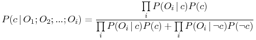
Bayesian statistics can provide an estimate of the probability of
association for each candidate.
Given multiple observables,  , that each provide some discrimination on
the two possibilities, either the star is a companion (c) or it is a field
star (ie, not c or
, that each provide some discrimination on
the two possibilities, either the star is a companion (c) or it is a field
star (ie, not c or  ), the standard Bayesian formula in this case is,
 |
(4) |
Where the numerator has the product of available probabilities for
each observable having its observed value assuming that the candidate
is a companion,  .
The numerator also includes a prior
probability term,
.
The numerator also includes a prior
probability term, ![]() , in which knowledge of the companion
probability of the ensemble of candidates or additional knowledge of the
companions can be introduced.
If no prior knowledge is available, then this term can be set
to
, in which knowledge of the companion
probability of the ensemble of candidates or additional knowledge of the
companions can be introduced.
If no prior knowledge is available, then this term can be set
to  , and at least one will have a rank ordering in the
probabilities of the candidates.
The denominator has a repeat of the
numerator, plus a similar product of probabilities, except this time
the assumption is that the candidate is not a companion.
, and at least one will have a rank ordering in the
probabilities of the candidates.
The denominator has a repeat of the
numerator, plus a similar product of probabilities, except this time
the assumption is that the candidate is not a companion.
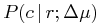
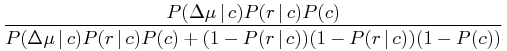
For this work, the discriminating observables are radial separations r from parallax, proper motion differences Δμ, so the above formula for the posterior probability of being a companion is:
 |
 |
 |
(5) |
With the prior P(c) set to 0.5 this provides probabilities with a starting assumption that each candidate is just as likely to be a field star as a companion. One can improve on this by providing the probability of being a companion based on statistics of the field stars that are nearby in angle, proper motion, and distance separation Δd.
 |
(6) |
Here, ![]() is the probability that one or more field stars
fall with radial distance less than the candidate's distance from the primary.
Therefore,
is the probability that one or more field stars
fall with radial distance less than the candidate's distance from the primary.
Therefore, ![]() is the probability that no field stars randomly fall
in this range.
The term
is the probability that no field stars randomly fall
in this range.
The term ![]() is the probability that one or more field
stars happens to have proper motion and angular separation more similar
to the primary than the candidate.
is the probability that one or more field
stars happens to have proper motion and angular separation more similar
to the primary than the candidate.
The term P(p) is the probability that the provisional primary, selected in the manner in which it has, is a primary, i.e., it has at least one wide companion in the radial region that we are exploring. It is perhaps somewhat dismaying at first that P(p) is needed to derive individual probabilities since normally the individual probabilities would be needed to derive it. However, as we show, it is possible to conduct control experiments, using the actual catalog data, to constrain P(p).
§ 3.1.1. P(Δ&mu | companion) and P(r | companion)
To calculate the probability that a binary star would have a given proper motion difference, one could calculate the intrinsic probability density function of velocities for random orbits from Kepler's Laws and take into consideration distances, errors in distances, and errors in proper motion observations. The probability of having some specified observed proper motion difference Δμ assuming it is a companion, is given by the complementary cumulative distribution function (CCDF) which is the integral of the PDF over proper motion differences greater than the observed value.
 |
|
 |
(7) |
However, it is more straightforward to create a simulation of the star catalog (discussed in § 3.3), add simulated binary orbits, add observational errors and then form the histogram of the distribution of proper motions. Per Eq. (7), the cumulative distribution is reversed and this provides estimates of the probability of a companion to have the observed proper motion value. These probabilities are fit sufficiently well by the following form for the components parallel and perpendicular to the motion of the primary:
 |
|
![\displaystyle\exp[{-(\mu _{{\perp}}/\mu _{0})^{{\alpha _{0}}}}],](mi/mi198.png) |
(8) | ||
 |
|
![\displaystyle\exp[{-(\Delta\mu _{{\parallel}}/\Delta\mu _{1})^{{\alpha _{1}}}}].](mi/mi45.png) |
(9) |
The probability that a companion would have both components greater than the observed ones is,
 |
|
 |
(10) |
The parallel and perpendicular coordinates are used here because our first-order error analysis indicates that most geometric effects will be parallel to the motion of the primary (see §§3.2 and Eq. (29) below).
For the probability based on radial distributions, we
calculate the period ![]() using
using ![]() and apply it to the CCDF of the DM91
distribution modified to allow for individual errors in parallax that
reflect into errors in r which then reflect into errors in the period of orbit.
The CCDF of this log-normal distribution is given by the complementary error function:
and apply it to the CCDF of the DM91
distribution modified to allow for individual errors in parallax that
reflect into errors in r which then reflect into errors in the period of orbit.
The CCDF of this log-normal distribution is given by the complementary error function:
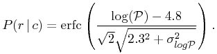 |
(11) |
Of course, for radial separations of several parsecs where the system is no longer bound the DM91 distribution looses meaning, but it continues to be useful in providing a steeply descending function.
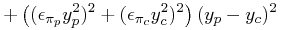
The error in r is given by:
 |
|
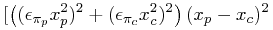 |
(14) | ||
 |
|||||
![\displaystyle+\left((\epsilon _{{\pi _{p}}}z_{p}^{2})^{2}+(\epsilon _{{\pi _{c}}}z_{c}^{2})^{2}\right)(z_{p}-z_{c})^{2}]/r^{2}](mi/mi157.png) |
But, we need the error in the log of the period due to uncertainty in distance,
 |
(15) | ||||
 |
(16) |
§ 3.1.2. P(Δμ,θ | field) and P(Δd | field)
We seek the probability that one or more field stars would have a proper motion as close or closer to the primary as the candidate given the local density if stars per unit spatial and proper motion area. The number density is given by:
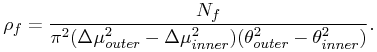 |
(17) |
The formula for the probability of one or more stars, chosen from a homogeneous distribution with this density, falling at separation less than θpair and proper motion difference less than Δμ is:
 |
|
 |
(18) |
Even though this formula is formally for a constant density distribution it works well for a density changing linearly in the coordinates. However, near the peak of the density distribution with proper motion along a line of site, the curvature in the density profile can cause substantial error in the local density and it is best to simply avoid this calculation near the peak. Since the peak is where the density becomes very high and probabilities are low, this region needs to be avoided anyway. Therefore, we only consider primaries with a field density below a given threshold (Table 1).
The probability that one or more field stars would happen to have an observed distance that is less than the Δd observed for a candidate star is given by similar formulae,
 |
|
 |
(19) | ||
 |
|
 |
(20) |
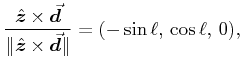
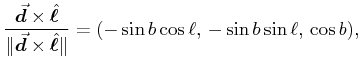
§ 3.2. Geometrically induced proper motion differences.
With increasing stellar separation there is a growth in the proper
motion difference caused by various projection effects, even if
the two stars have the same space motion. However, in most cases
some compensation can be made for this. We can first look mathematically at the
gradient of  due to spatial separations at
constant space velocity.
To search for very wide binaries, we start by presuming space velocities
are essentially the same for the sytem's stars.
For a binary with a solar mass primary separated by more than 0.01 pc,
the orbital velocities are
< 0.78 km s-1.
Beyond 25 pc, this corresponds to < 6.6 mas yr-1 in
proper motion differences.
In Galactic coordinates
due to spatial separations at
constant space velocity.
To search for very wide binaries, we start by presuming space velocities
are essentially the same for the sytem's stars.
For a binary with a solar mass primary separated by more than 0.01 pc,
the orbital velocities are
< 0.78 km s-1.
Beyond 25 pc, this corresponds to < 6.6 mas yr-1 in
proper motion differences.
In Galactic coordinates  , the vector of
proper motion is composed of the two projections of the 3-d velocity onto
the unit vectors in the longitude and latitude directions, divided by
the distance d to the star.
, the vector of
proper motion is composed of the two projections of the 3-d velocity onto
the unit vectors in the longitude and latitude directions, divided by
the distance d to the star.
|
 |
(21) | |||
 |
|
 |
(22) | ||
 |
|
 |
(23) | ||
 |
|
 |
(24) | ||
 |
|
 |
(25) | ||
 |
|
 |
(26) |
where  is the unit vector to the North Galactic Pole.
If distances are in pc and proper motions are in
is the unit vector to the North Galactic Pole.
If distances are in pc and proper motions are in  , then the radial
velocities are in AU yr
, then the radial
velocities are in AU yr (1 AU yr
 ).
The velocity
).
The velocity  is
relative to the sun so it is formally ⋅
is
relative to the sun so it is formally ⋅
 , where
  is the
velocity of the sun in the Local Standard of Rest (LSR).
is the
velocity of the sun in the Local Standard of Rest (LSR).
The derivatives of the direction vectors:
|
 |
(27) | |||
 |
|
 |
(28) |
can be used to derive the gradients in spherical coordinates to get a first order assessment of the geometric induced variations on the difference in proper motion between two stars moving at the same space velocity:
 |
|
 |
(29) |
where  and
and  are the difference in longitude and
latitude, in radians.
Similarly, we can look at the first derivatives of the radial velocity
which, if known for both components, can be taken into account when
assessing whether the pair is really co-moving:
are the difference in longitude and
latitude, in radians.
Similarly, we can look at the first derivatives of the radial velocity
which, if known for both components, can be taken into account when
assessing whether the pair is really co-moving:
 |
|
 |
(30) |
As an example, let us examine a case where  ,
,  , the radial velocity is -20 km s-1, the primary's
distance is 20 pc, the companion is 1 pc farther away than the primary,
and they are separated by 1 degree per coordinate (
, the radial velocity is -20 km s-1, the primary's
distance is 20 pc, the companion is 1 pc farther away than the primary,
and they are separated by 1 degree per coordinate ( , separation
½ pc ). We then have:
, separation
½ pc ). We then have:
 |
|
 |
||
 |
|
 |
||
|
|
 |
Note that the changes in proper motions can be quite significant
with respect to the measurement errors (typically 1 – 3  and 1 – 3
km s-1).
This implies that very wide binaries of several degrees in separation are,
in general,
not found by commonality in proper motions, unless proper geometric corrections have been applied.
and 1 – 3
km s-1).
This implies that very wide binaries of several degrees in separation are,
in general,
not found by commonality in proper motions, unless proper geometric corrections have been applied.
Eq. 29 implies that when relative distances are unknown, one
can still make useful corrections using the proper motions and radial
velocities. And, when radial velocities are also unknown one can still make
useful corrections, by assuming  , that become highly accurate for
 near the poles.
Also, one can mitigate somewhat against large uncertainty in the
 term in Eq. (29), by taking note that
this term is parallel to a system's overall proper motion.
Therefore, one should treat the parallel and
perpendicular components of the proper motion separately to take
advantage of the
perpendicular component which needs no correction term and hence is less noisy.
term in Eq. (29), by taking note that
this term is parallel to a system's overall proper motion.
Therefore, one should treat the parallel and
perpendicular components of the proper motion separately to take
advantage of the
perpendicular component which needs no correction term and hence is less noisy.
The first order correction, Eqs. (29), is typically good
to < 10% for angles < 5° and distance differences of < 30%,
except near  where the term goes to zero for changes in angle.
To explore out to separations of ≈10° and reach several pc physical separations,
a full (nonlinear) correction for space velocities is made.
We calculate the 3-d space velocity of each primary
from its proper motion and radial velocity (Eqs. 31 –
33), if we have it,
and, using Eqs. (24) – (25), calculate the
proper motion that this space motion implies, if it were in the
direction of each companion candidate.
If there is no radial velocity for the primary, then the system is
assumed to be at rest in the LSR.
In those cases, the projection of the
the Solar Motion in the radial direction is subtracted,
using (10.0, 5.25, 7.17) km s-1> for the Solar Motion.
As described in § 4.1, for
where the term goes to zero for changes in angle.
To explore out to separations of ≈10° and reach several pc physical separations,
a full (nonlinear) correction for space velocities is made.
We calculate the 3-d space velocity of each primary
from its proper motion and radial velocity (Eqs. 31 –
33), if we have it,
and, using Eqs. (24) – (25), calculate the
proper motion that this space motion implies, if it were in the
direction of each companion candidate.
If there is no radial velocity for the primary, then the system is
assumed to be at rest in the LSR.
In those cases, the projection of the
the Solar Motion in the radial direction is subtracted,
using (10.0, 5.25, 7.17) km s-1> for the Solar Motion.
As described in § 4.1, for  pc, there are
radial velocity measures for most of the primaries.
pc, there are
radial velocity measures for most of the primaries.
The conversion to space velocities is the inverse of Eqs. (24) – (26) and has solution:
 |
|
 |
(31) | ||
 |
|
 |
(32) | ||
 |
|
 |
(33) |
To avoid excessive error arising from distance uncertainties at distances beyond 25 pc, we assume the companion is at the distance of the primary.
§ 3.3. Simulation
A program for creating simulations of the Solar Neighborhood distribution of stars with binary systems was written to test the methodology, search for optimal parameters, and to understand the origin and behavior of false positives. The simulations cover a large range of parameters to understand the reliability and broadness of applicability of the methodology. The simulations also are used as a quick way to derive the shape of the cumulative distribution functions for the observables in an ensemble of random binary systems.
In a simulation, stars are set down with a distribution of positions
and velocities that statistically imitate the
HIP2 after observational errors are included.
Masses are distributed with the power law  from 0.8 to 15
  and luminosities
follow a mass-luminosity relation,
and luminosities
follow a mass-luminosity relation,  .
An arbitrary fraction of the stars are given companions.
The companions do not themselves
host companions, e.g., no hierarchical systems are created.
The orbital elements: eccentricity, inclination, longitude of the ascending node,
longitude of the periapsis, and epoch are
random uniform distributions.
The distribution of periods is chosen to be log-normal without a long period cutoff.
.
An arbitrary fraction of the stars are given companions.
The companions do not themselves
host companions, e.g., no hierarchical systems are created.
The orbital elements: eccentricity, inclination, longitude of the ascending node,
longitude of the periapsis, and epoch are
random uniform distributions.
The distribution of periods is chosen to be log-normal without a long period cutoff.
We first present the relatively small false positive rate for a simulation in
which no binary stars were generated.
In Fig. 1 the numbers of companions with probabilities >0.1 vs.
angular separation are shown (thick black solid line),
where the associated primaries are in the 25 – 50 pc (left) and
50 – 100 pc (right) distance ranges .
The “false positive” rate is kept low by using a low value for the prior
 , namely 0.20 for 25 – 50 pc and 0.07 for 50 – 100 pc.
These values for are chosen because they work reasonably well for all that follows.
, namely 0.20 for 25 – 50 pc and 0.07 for 50 – 100 pc.
These values for are chosen because they work reasonably well for all that follows.
Fig. 2 shows results of an analysis of a
simulation in which the semi-major axes are set by the DM91 distribution of periods
but using only periods longer than the peak of the distribution at 173 yr.
About 21% of the stars are primaries and 28% are companions.
These rates are much higher than the observed one, considering that the mass
function only goes down to 0.8 ,
but it provides many companions and much confusion to better test the procedure.
The primaries have 1, 2, 3, or 4 companions with frequency of roughly 67.8,
27.4, 4.5, and 0.2%, respectively.
The dotted green line shows the number of companions created per separation bin.
The solid thick line shows the number of companions found with probabilities
>10%.
The green solid line gives the number of correct primary-companion
associations found.
The lower green dashed line gives the number of companions ascribed to be
primary-companion pairs, but neither was
an input primary, i.e., it gives the number of secondary-tertiaries pairs, etc. found.
The procedure recovers better than 90% of the multiple systems for
separations out to 2° for
25 – 50 pc and 1°for 50 – 100 pc or about a parsec.
In Fig. 3 , the period distribution for the simulation is multiplied by 100 to shift the distribution to larger semi-major axes. Now, one can see that there is still reasonable recovery > 20%) of companions even at separations of 10° for 25 – 50 pc region and 5° for 50 – 100 pc. For 0 – 25 pc, we get good fractional recovery until 20°.
The resulting distributions of observables for this simulation are used
to set the coefficients presented in Table 1.
These coefficients do not depend on the fraction of stars that hold binaries,
nor do they depend strongly on the shape of the separation distribution.
They do depend fairly strongly on the assumed observational errors which essentially
determine the widths of the cumulative distributions.
However, as the width of the distributions change, the value of needs to adjust
in a direction to keep the sum of the probabilities constant near the values
indicated by the control experiments (next section).
The net result is that the assigned probabilities
change rather slowly with the observational errors assumed.
Since this paper presents a quick test of the methodology, just a single set of
observational errors representative of moderately faint stars in TY2 are used:
σμ = 1.5 mas yr-1 ,
![]() 1 mas. For parallax, we use
σπ = 1 mas to represent the HIP2 data.
This turns out to be sufficient for the task, for now.
1 mas. For parallax, we use
σπ = 1 mas to represent the HIP2 data.
This turns out to be sufficient for the task, for now.
§ 3.4. Control Experiments
We implement two kinds of control experiments that use the observed data
directly
rather than the simulation to assess the rate of false positives and
thereby determine the prior probability . Using the real
data for control tests provides greater confidence that minor
differences between the simulation and reality do not cause
inconsistencies. In the first method, the negative of the
Galactic latitude is used for each star while it is considered as a primary.
This moves the primary away from its companions and places it in a
region with similar stellar density and velocity field. Any
stars assigned high probabilities are statistical coincidences or false
positives.
Although there is asymetry between the two hemispheres in the observed
proper motion distribution, much of this goes away after transforming to
the LSR and the remaining should have a small affect on the numbers of
false positives.
In the second method, all candidates are removed from each primary, and then each field star is randomly “rethrown” with new uniform random 2-d positions within the separation angle limit, θouter, and random values of Δμ within a circle in coordinates (Δ&mu||, Δμ⊥) whose size is set to maintain the density in phase-space. The field star distances and brightnesses are maintained. When the control experiments are run on a simulation with zero binaries, the two control methods and the direct analysis of the simulation returns approximately the same number of false positives, within each probability bin, as they should. The first method of control experiment, with the reverse sign of b value of each primary, is shown as blue triangles in Fig. 1, where no binary stars are generated in the simulation. The second method, with field star rethrown, is shown as blue squares with error bars at the average and rms deviations of 4 realizations. For the other figures showing number versus separation, both types of control experiments are averaged together and shown as blue squares.
§ 4. Application to the Hipparcos Catalogue
As a first application of our Bayesian probability estimator,
Eqs. (5) and (6), we examine stars in the
HIP2 brighter than 10th mag in V-band for possible
companion stars brighter than V=12.
Provisional primaries are separated into three distance
intervals, by parallax distance. There are 1,041 potential primaries
(V 10) within 25 pc, 4,152 in the 25 – 50 pc shell,
and 14,064 in the 50 – 100 pc shell.
A 15° radius around the Hyades is cut out when working with the 25 – 50 pc
primaries.
A 200′ radius around the Pleiades Cluster and also
around the Coma Star Cluster are cut out for 50 – 100 pc primaries.
Stars with
10) within 25 pc, 4,152 in the 25 – 50 pc shell,
and 14,064 in the 50 – 100 pc shell.
A 15° radius around the Hyades is cut out when working with the 25 – 50 pc
primaries.
A 200′ radius around the Pleiades Cluster and also
around the Coma Star Cluster are cut out for 50 – 100 pc primaries.
Stars with  mas are presumed to be too far away and are also
removed. For companions, about 25,000 stars are brighter than V=12
and are within 110 pc.
mas are presumed to be too far away and are also
removed. For companions, about 25,000 stars are brighter than V=12
and are within 110 pc.
Candidate companions and field stars are selected if their separation from the primary is 36″ < θlim < 20° for dp < 25 pc, 36″ < θlim < 20° for 25 < dp < 50 pc, and 18″ < θlim < 20° for 50 < dp < 100 pc, (Table 1). Most HIP binaries closer than 36″ and within 50 pc would already be known and their proper motion differences may be substantially affected by orbital motion, while our methodology is optimized for the case of low orbital speeds. Companions are not constrained to come from the same distance interval as the primary star. Table 2 presents how many potential primaries there were in each distance range and the numbers remaining after dropping ones with no stars nearby, then no candidates, then too high of a field density, and finally presents the number of primaries and candidates with probabilities over 0.1. The total probabilities given for all candidates in the entire separation range and for just those with separations < 1 pc.
Table 1 provides the final set of parameters that are used in the analysis of each distance intervals and in creating the tables and figures in this section. In addition to the coefficients for the cumulative distributions in each of the observables and the cutoffs in angle and proper motion for candidates and for field star counts, the table includes the maximum number of field stars accepted. Most field stars along a given direction are concentrated in a small range of proper-motion: consistent with expectation from the Galactic rotation and the projection of the Solar Motion along the line-of-sight. If the phase-space of the star is well centered in this “cloud”, usually, the probabilities for any companions would naturally be low and the rate of false positives unacceptably high. To avoid this a star is dropped if the field phase-space density is in the 90-percentile in the density distribution. However, in the 0 – 25 pc region, the number of candidates is always small, so, it is unnecessary to include this criterion there.
Histograms of the separation distributions for the HIP
are shown in Fig. 4 (in degrees) and
Fig. 5 (in parsecs) for probabilities of "> 0.1.
In each diagram, the thick black line is the
histogram of companions with the chosen probabilities, the blue
square symbols are the averages over 5 control experiments, and the red
lines shows the numbers found minus the numbers in the control experiments,
providing an estimate of the range of real physical companions (red error bars).
This choice for is simply the value that brings the sum of the
probabilities in each bin into agreement with
the number of companions found minus the number in the control experiments.
The sum of the probabilities of companions within each separation bin
(thick purple dash-dotted line) has been adjusted by varying ,
settling at a value of 0.20 for 25 – 50 pc and 0.07 for 50 – 100 pc.
The degree of agreement is startling to the authors.
Since the actual distribution at these separations is very different
from the DM91 distribution used in  ,
one might worry that it would not work at all.
However, all that is required
for this probability is a function that falls off rapidly enough to
sufficiently suppress the false positives, and the DM91 law happens to work.
,
one might worry that it would not work at all.
However, all that is required
for this probability is a function that falls off rapidly enough to
sufficiently suppress the false positives, and the DM91 law happens to work.
For separations up to ≈ 1 pc the number of false positives found in the control sample is quite small implying that the companions found in the real sample are reliable. The breakdown by probability interval at various separations is presented in Fig. 6; the different colored regions show the distribution contoured at 0.1, 0.25, 0.75, and 0.95 probability levels.
§ 4.1. Radial Velocities
Radial velocities differences can be used, where available, as a check on the
reasonableness of the probability assignments; therefore we searched the
literature for radial velocity measures of HIP stars.
Because some radial velocity (RV) catalogs in CDS4
-
The SIMBAD data base. While we did extract the radial velocities in batch mode, the errors could not be obtained in that way. So all RV errors for these stars are set to 10 km s-1. We find 36,884 HIP stars with RV data in SIMBAD.
-
The General Catalogue of Mean Radial Velocities [GCRV; Barbier-Brossat & Figon (2000); SIMBAD cat. III/213]; following the description in SIMBAD catalog III/21 (Wilson, 1953), the following values for the RV errors based on the quality factors are assigned: quality=A →εRV = 0.5 km s-1, q=B →εRV = 1.2 km s-1 , q=C →εRV =2.5 km s-1, q=D →εRV = 5.0 km s-1. Stars with quality E (εRV > 20 km s-1) are excluded. These errors correspond more or less to the midpoints of the ranges specified by Wilson (1953). We find 21,120 HIP stars in the GCRV.
-
The Bibliographic Catalogue Of Radial Velocities [BCRV; Malaroda et al. (2000); SIMBAD cat. III/249], which is up to date till 2006. This catalog required significant attention as it does not list errors on the RVs, while also many stellar names do not conform to the current SIMBAD convention. This may not be too surprising since Malaroda et al. (2000) compiled RV data from almost 1300 different publications. However, the vast majority of stars are found in just 33 different publications. We read those 33 publications and estimated an RV error for each of them. Stars from other publications are, somewhat arbitrarily assigned RV errors of 10 km s-1. 1,178 stars are found in more than one publication, and their weighted average values and errors are used in our database. In total, we find 14,279 HIP stars in the BCRV that are not in the GSCN catalog, described below.
-
The Catalogue of Radial Velocities of Galactic Stars with Astrometric Data, the Second Version [CRVAD; Kharchenko et al. (2007); SIMBAD cat. III/254]. The same error assignment is used here as for the GCRV above, and stars with RV quality=E are not used. We find 41,740 HIP stars in the CRVAD.
-
The Geneva-Copenhagen Survey of the Solar Neighborhood [GCSN; Nordström et al. (2004); SIMBAD cat. V/1175
The original catalog V/117 is hard to find on SIMBAD because it is claimed to be obsoleted by V/130. However, V/130 contains significantly less information, i.e., neither mass estimates nor the raw RV information. This catalog can be accessed by going directly to the source: http://vizier.u-strasbg.fr/viz-bin/VizieR?-source=V/117.]. The “median errors” as listed in the GCSN are used. We find 11,900 HIP stars in the GCSN that were not taken from the GCRV. -
The Radial Velocity Experiment: Second Data Release [RAVE; Zwitter et al. (2008); SIMBAD cat. III/257]. We use the errors as presented in the RAVE catalog. If more than one entry is present per HIP star, the weighted average for both the value and the error are used. We find 393 HIP stars in the RAVE data set.
Altogether, we have 43,047 radial velocities out of 113,942
HIP stars with positive parallaxes: the average completeness is 37.8%.
The additional catalogs added 6,161 RVs to that available in SIMBAD alone.
The completeness fraction is a strong function of distance
(Fig. 9) and apparent magnitude.
About 48% of
stars at a distance of 100 pc have a measured radial velocity, but
within 100 pc, RV data is available for almost two-thirds of stars.
Of the systems where both
the primary and candidate have a measured RV,  87% systems have
errors 10 km s-1, with an average of about 1.5 km s-1.
87% systems have
errors 10 km s-1, with an average of about 1.5 km s-1.
For those stars with RV data in multiple catalogs, we compared the various values to assess their external accurcy. If a star is in fact a binary, then the cataloged values might have been taken at different orbital phases, which would result in a scatter that is larger than expected on the basis of the reported internal errors. We kept track of the range of the reported RVs for a given star, and the errors. If this range exceeds 1.6 times the error and the velocity range exceeds 9 km s-1, then the star is deemed to have a discrepant RV, which may be the result of (unsuspected) binarity. About 13% of HIP stars are classified as some sort of binary, while the ones with discrepant radial velocities are classified as binaries about four times more often (≈55%). For our subsample of candidate very wide binaries with discrepant RVs, about 75% are known or suspected binaries. The whole sample of very wide binary candidates has a rate of known/suspected binaries that is 3x larger than for the whole HIP. It is important to note that these known/suspected binaries most often refer to companions closer to our candidates, not the candidates we report in this paper. We interpret this as evidence that very wide binaries are often found in hierarchical systems, as suggested by a number of authors (Makarov et al., 2008; Caballero, 2009, 2010; Kouwenhoven et al., 2010).
§ 4.2. Stellar Masses
It's useful to obtain mass estimates for the stars in these systems to learn
how their separations compare with their nominal tidal radii.
Absolute magnitudes ( ) and
stellar masses (
) and
stellar masses ( ) are assigned based solely on stellar color (B-V),
via the mass-luminosity-color relation for the main-sequence (MS).
We note that the so-determined
) are assigned based solely on stellar color (B-V),
via the mass-luminosity-color relation for the main-sequence (MS).
We note that the so-determined  relation forms a lower envelope to
the HIP color-magnitude diagram for main-sequence stars: our relation is
close to, but not identical to the zero-age main sequence (ZAMS)
relation.
The starting point is Tables 3.13 and
3.10 in Binney & Merrifield (1998), which list stellar colors, masses and absolute
magnitudes as a function of spectral type. Next,
the colors are updated in the following way.
1) The BVRI colors for O5
– M5 stars are taken from Cox (2000), where this
source is also used for the values of effective temperature (
relation forms a lower envelope to
the HIP color-magnitude diagram for main-sequence stars: our relation is
close to, but not identical to the zero-age main sequence (ZAMS)
relation.
The starting point is Tables 3.13 and
3.10 in Binney & Merrifield (1998), which list stellar colors, masses and absolute
magnitudes as a function of spectral type. Next,
the colors are updated in the following way.
1) The BVRI colors for O5
– M5 stars are taken from Cox (2000), where this
source is also used for the values of effective temperature ( ).
2) BVRI colors are preferentially taken from Bessell (1990) for types
M0 – M6.
3) The previous references are superseded by VRIJHK data from
Bessell (1991) for
M6 – M7.5 dwarfs.
4) Average B-V colors are computed for
late-type M dwarfs by averaging the colors and of several such dwarfs
extracted from the NSTARS
database6
).
2) BVRI colors are preferentially taken from Bessell (1990) for types
M0 – M6.
3) The previous references are superseded by VRIJHK data from
Bessell (1991) for
M6 – M7.5 dwarfs.
4) Average B-V colors are computed for
late-type M dwarfs by averaging the colors and of several such dwarfs
extracted from the NSTARS
database6 0.064, 1.99
0.009, 2.05 0.078, 2.16 0.8 and 2.10 for
types M5.5, M6.0, M6.5, M7.0 and M8.0, respectively.
0.064, 1.99
0.009, 2.05 0.078, 2.16 0.8 and 2.10 for
types M5.5, M6.0, M6.5, M7.0 and M8.0, respectively.
For all cases, we use the dependence of a given color on to
interpolate over missing values8 = 0.85 (B-V)
 . This transformation is
accurate to 0.071 mag, which is 2.2 times larger than the
errors on B-V as listed in HIP. Note that we use the TY2 colors,
which differ substantially (at fainter magnitudes) from the TY1
colors listed in HIP.
. This transformation is
accurate to 0.071 mag, which is 2.2 times larger than the
errors on B-V as listed in HIP. Note that we use the TY2 colors,
which differ substantially (at fainter magnitudes) from the TY1
colors listed in HIP.![]() ,
, ![]() ,
,
![]() ,
,
![]() ,
,
![]() ,
,
![]() ,
, ![]() and
and
![]() 9
9
Lastly, a correction is made for the effects of stellar
evolution as stars evolve off the zero-age main sequence.
The GCSN catalog
(Nordström et al., 2004) provides stellar masses corrected for stellar
evolutionary effects, absolute magnitudes and  colors for
14,955 HIP stars. We compute a two-dimensional look-up table (map),
with the average mass as a function of (B-V) and .
This contour map, Fig. 10, shows for any star that
falls in a defined part of the map, the corresponding mass value used.
For stars in undefined parts of the map,
the color-mass relation for the MS is used.
The masses are listed in column #14 of tables
3 – 5.
Note that these masses
are insufficient to decide whether or not a potential pair is
bound because, quite often, the system contains stars that are not a
part of HIP.
colors for
14,955 HIP stars. We compute a two-dimensional look-up table (map),
with the average mass as a function of (B-V) and .
This contour map, Fig. 10, shows for any star that
falls in a defined part of the map, the corresponding mass value used.
For stars in undefined parts of the map,
the color-mass relation for the MS is used.
The masses are listed in column #14 of tables
3 – 5.
Note that these masses
are insufficient to decide whether or not a potential pair is
bound because, quite often, the system contains stars that are not a
part of HIP.
§ 4.3. Tabulated Results
The focus of this research has been on very wide companions in
the 25 – 100 pc interval; however, we
have applied a similar methodology to the 0 – 25 pc interval even though
it has not been optimized for this regime.
Fortunately, a number of high probability companions are discovered in
this region out to 20° in separation.
The physical systems and their probabilities are presented in tables
3, 4 and 5 for the distance
ranges 0 – 25 pc, 25 – 50 pc and 50 – 100 pc, respectively.
The names (columns #1 & #2), positions (cols. #3 & #4) and the
visual magnitude (col. #5) are taken from HIP. The spectral type
(#6) is taken from SIMBAD10
The proper motions (#7 & #8) are from TY2 when available,
otherwise they are from HIP2.
Columns #9 and #10 list the proper motions differences corrected for
geometric effects as described in
§3.2 above.
In detail, our procedure is as follows. First, for each
potential companion star, its space velocities  is computed
according to Eqs. (31 – 33) using their angular
coordinates, distances, and proper motions. However, beyond 25 pc,
the distance of the primaries is used because
is computed
according to Eqs. (31 – 33) using their angular
coordinates, distances, and proper motions. However, beyond 25 pc,
the distance of the primaries is used because  is meant to give the probability of having
  assuming
that it is a companion, and should not be reduced by a large distance error.
Beyond ~25 pc, the typical parallax errors,
imply distance errors that significantly
exceed the orbit size and would artificially inflate the
inferred proper motion corrections.
We use the RV of the primary because it is usually the better studied and,
therefore, is more likely to provide the barycentric velocity of the system.
assuming
that it is a companion, and should not be reduced by a large distance error.
Beyond ~25 pc, the typical parallax errors,
imply distance errors that significantly
exceed the orbit size and would artificially inflate the
inferred proper motion corrections.
We use the RV of the primary because it is usually the better studied and,
therefore, is more likely to provide the barycentric velocity of the system.
In the next step, these space velocities are transformed into
the expected proper motions if it were at the position of the primary.
The corrected proper motion
differences listed in columns #9 and #10 are the difference between
the proper motion components of the primary and the candidate if it were seen
with the same projections onto the sky as the primary.
In the same columns, the errors on
these  values are listed, which are derived via propagating
the errors on the observables. The procedure inflates the observed
proper motion errors, typically by factors of 2 to 4. This is to
be expected because the corrected proper motion difference
contains 3 or 4 terms (cf. Eq. [29])
that are RSS-ed together to yield the errors.
values are listed, which are derived via propagating
the errors on the observables. The procedure inflates the observed
proper motion errors, typically by factors of 2 to 4. This is to
be expected because the corrected proper motion difference
contains 3 or 4 terms (cf. Eq. [29])
that are RSS-ed together to yield the errors.
The distance (#11) is the inverse of obtained from HIP2.
Column #12 contains the radial velocities compiled in
§4.1.
For Column #13, the proper motion and radial velocity of the companion are
transformed to LSR space velocities at its position and then the radial
velocity is calculated from that space velocity translated to the position
of the primary.
Beyond 25 pc, we again use the primary's distance in the first step
instead of the companion's to minimize correction errors due to
distance uncertainties.
The errors on the corrected RVs are nearly the same as the errors on the
measurements themselves because the corrections are typically small.
The RV differences are plotted in Fig. 8.
The separation (#15) follows from the positions of the
primaries and companions and the distance of the primary.
Column #16 gives the probability of the candidate being a true companion of the primary according to Eq. (5).
The last column (#17) provides Bayer-Flamsteed (BF) designations and common names for the stars. These are extracted from the “HD-DM-GC-HR-HIP-Bayer-Flamsteed Cross Index” (Kostjuk, 2004), with the following modifications: 1) a common name is not listed if the same name is used for another HD star, unless the system is a close pair, 2) if more than one common name was specified, the shortest one is used. Note that in some cases, Kostjuk (2004) uses as the BF designation both the numeric and the Greek designation. If the star has another HIP star as a companion (as listed in HIP), we add the known HIP numbers after the “kn:” designation.
§ 4.4. Some Notable Companion Pairs
We find these unnoticed naked-eye companions (6 mag):
Capella & 50 Per,
mag):
Capella & 50 Per,  Vel & HIP 43797,
Alioth (ε UMa), Megrez (δ UMa) & Alcor (80 UMa),
γ & τ Cen, φ Eri & η Hor, 62 & 63 Cnc,
γ & τ Per, ζ & δ Hya,
β01, β02 & β03 Tuc, N Vel & HIP 47479,
HIP 98174 & HIP 97646, 44 & 58 Oph, s Eri & HIP 14913,
and &
Vel & HIP 43797,
Alioth (ε UMa), Megrez (δ UMa) & Alcor (80 UMa),
γ & τ Cen, φ Eri & η Hor, 62 & 63 Cnc,
γ & τ Per, ζ & δ Hya,
β01, β02 & β03 Tuc, N Vel & HIP 47479,
HIP 98174 & HIP 97646, 44 & 58 Oph, s Eri & HIP 14913,
and &  Cep.
High probabality fainter companions (> 6th mag) of stars
Cep.
High probabality fainter companions (> 6th mag) of stars  are found for:
Fomalhaut (α PsA), γ UMa, α Lib, Alvahet (ι Cephi),
δ Ara, Chow (β Ser), ι Peg, β Pic, κ Phe. and
γ Tuc
are found for:
Fomalhaut (α PsA), γ UMa, α Lib, Alvahet (ι Cephi),
δ Ara, Chow (β Ser), ι Peg, β Pic, κ Phe. and
γ Tuc
§ 4.4.1. The Capella System
We identify the T Tauri star 50 Per (HIP 19335) as
a P = 0.2 candidate companion of Capella.
While these stars have almost
equal radial velocities and corrected proper motion differences,
they are separated by almost 15° on the sky (5.4 pc) and have a 3D separation
of 8.9 pc.
The corrected proper motion differences (~12 ± 5 mas
yr-1) may seem a bit too large to accept this system as a real
wide-binary candidate, but this difference is time dependent.
Capella is an almost equal-mass spectroscopic binary with component
masses 2.466 & 2.443 .
It has, 12′ away, known companion WDS 05167+4600 HL which
comprises the M1V star GJ 195 A (V=10.16 mag) and the M5 dwarf
GJ 195 B (V=13.7 mag), which are separated by 6″.
50 Per itself is paired here with HIP 19255 at a
separation of ~15,200 AU (~740″). Furthermore, the MSC
identifies both 50 Per and HIP 19255 as possible binaries
themselves, while these systems orbit each other in about one
million years at an equivalent circular orbit speed of  0.45
km s-1 (4.8 mas -1). The MSC reports a total mass 3.64 for the
50 Per and HIP 19255 system. The two components of HIP 19255 are
separated by 3
0.45
km s-1 (4.8 mas -1). The MSC reports a total mass 3.64 for the
50 Per and HIP 19255 system. The two components of HIP 19255 are
separated by 3 87 and orbit each other in 590 years
(vorb ≈ 4 km s-1 = 42.5 mas
yr-1). This orbital speed is more
than sufficient to account for the corrected proper motion
difference between 50 Per and HIP 19255. We find the following about
the putative 50 Per binary: 1) The HIP2 and TY2 proper motions for
50 Per differ by 2.7 ±1.7 mas yr-1, 2) HIP finds an acceleration
in the proper motion which Makarov & Kaplan (2005) estimate to
be 5.8 ± 3 mas yr-2
(
87 and orbit each other in 590 years
(vorb ≈ 4 km s-1 = 42.5 mas
yr-1). This orbital speed is more
than sufficient to account for the corrected proper motion
difference between 50 Per and HIP 19255. We find the following about
the putative 50 Per binary: 1) The HIP2 and TY2 proper motions for
50 Per differ by 2.7 ±1.7 mas yr-1, 2) HIP finds an acceleration
in the proper motion which Makarov & Kaplan (2005) estimate to
be 5.8 ± 3 mas yr-2
(![]() 0.5 km s-1
yr-2), and 3) the GCSN reports 8 oservations
over a period of 7 years with measurements errors of 0.2 km s-1 and
an ensemble error of 0.6 km s-1: this is consistent with an
acceleration of 0.286 ± 0.06 km s-1 yr-2. Thus, both RV and proper
motion data indicate the presence of an unseen companion for 50 Per.
The corrected proper motion and RV differences between
50 Per and Capella are bridged at the observed accelerations of
50 Per after 4 ± 3 and 17 ± 4 years, respectively.
0.5 km s-1
yr-2), and 3) the GCSN reports 8 oservations
over a period of 7 years with measurements errors of 0.2 km s-1 and
an ensemble error of 0.6 km s-1: this is consistent with an
acceleration of 0.286 ± 0.06 km s-1 yr-2. Thus, both RV and proper
motion data indicate the presence of an unseen companion for 50 Per.
The corrected proper motion and RV differences between
50 Per and Capella are bridged at the observed accelerations of
50 Per after 4 ± 3 and 17 ± 4 years, respectively.
The total mass for the Capella/50 Per system is (5.88+3.64)=9.52
![]() , so that the Jacobus radius is 2.8 pc, or about three times
smaller than the observed separation. Thus, Capella and 50 Per may
be an example of an escaped binary system.
, so that the Jacobus radius is 2.8 pc, or about three times
smaller than the observed separation. Thus, Capella and 50 Per may
be an example of an escaped binary system.
Although we also list the known double, HIP 26779 and HIP 26801, at 509′ or 2 pc from Capella as having very high probability for being physically related to Capella, unless the radial velocity is just wrong, we suspect that these are false positives. The barycentric velocity is well established, therefore the ~25 km s-1 difference in radial velocities is hard to explain unless this system is just passing by.
§ 5. Conclusions
We have applied a full Bayesian approach to assigning probabilities of companionship between HIP stars separated by more than 0.01 pc. By companionship we mean either bound gravitationally as in a system of small numbers of stars or co-moving with nearly the same velocity as in an escaped previously bound component. After subtracting the expected numbers of false positives derived from control experiments, a population of companions extending out to 8 pc in separation remains. Some of these very wide systems contain hierarchies of fairly massive stars that extend the tidal radii out to unusually large distances, but it is likely that others are recently unbound systems that continue to travel along nearly the same trajectory. While some of these seem to be parts of known nearby moving clusters or associations (e.g., Tucanae Stream, Hyades Stream, UMa Moving Cluster, β Pic Moving Group, and TW Hydrae Association), this procedure brings to focus even higher density knots within them, which should be far more persistant than the rest of the association either as a bound system or a tight stream. The amount of time after breakup of an open cluster or binary system for which companions stay in close proximity may be an important constraint on the mass and distribution of dark matter candidates such as dark subhalos.
Our statistical method finds both many highly significant pairings that
are missed by previous techniques and assigns reasonable probabilities for
companions even in regions previously considered too complicated or
crowded.
In the 1 – 100 pc distance range, we find altogether ![]() 34 companions with separations
0.01 – 1 pc and
34 companions with separations
0.01 – 1 pc and ![]() 50 companions with separations 1 pc – 8 pc.
Our preliminary investigations do not show any obvious trend for the
excess of wide/escaped
binaries along the Galactic rotation direction.
50 companions with separations 1 pc – 8 pc.
Our preliminary investigations do not show any obvious trend for the
excess of wide/escaped
binaries along the Galactic rotation direction.
As displayed in Fig. 8, we find good
agreement between the radial velocities of the primary and the
corrected RV of the candidate companions: 56% have velocity
differences  km
s-1 (about 3σ). For comparison,
the distribution of RV differences of random nearby HIP-HIP
pairs closely resembles a zero-centered Gaussian with a dispersion
of
km
s-1 (about 3σ). For comparison,
the distribution of RV differences of random nearby HIP-HIP
pairs closely resembles a zero-centered Gaussian with a dispersion
of ![]() 37.5 km s-1, which leads to a 15.8% chance that a random pair
would have a velocity difference as small as 6.8 km s-1. In addition,
unresolved spectroscopic binaries can induce RV differences of
order 10 – 30 km s-1, and so pairs with substantial RV differences
might in fact be physically associated. Therefore, the fraction of pairs
with small true RV differences could be significanly higher.
37.5 km s-1, which leads to a 15.8% chance that a random pair
would have a velocity difference as small as 6.8 km s-1. In addition,
unresolved spectroscopic binaries can induce RV differences of
order 10 – 30 km s-1, and so pairs with substantial RV differences
might in fact be physically associated. Therefore, the fraction of pairs
with small true RV differences could be significanly higher.
In some individual cases, such as Capella two of its candidate companions (HIP 26779 & 26801), the RV data indicates that the candidates are not real. Out of 426 candidates with radial velocities, we find 187 (44%) pairs for which the corrected radial velocities deviate by more than three times the errors: most of these systems might qualify as false positives. This rate of potential false positives agrees excellently with the rate identified in the control experiments (Fig. 5 and Table 5) of 428 control candidates out of 964 HIP candidates or 44%.
Figs. 2 and 4 indicate that the classical log-normal period distribution (DM91) results in a distribution of pair separations that is very different from the one we observe. To double check this, we use another simulation, where each HIP star is assigned a secondary with a mass drawn from the initial mass function. The absolute magnitudes for these simulated stars are estimated by applying the inverse of the procedure outlined in §§4.2 above. We then use the magnitude-completeness function of HIP to decide to accept or reject a given simulated secondary. While this procedure more-or-less reproduces the number of known HIP-HIP binaries, the distribution of separations resembles the results obtained from our simulation (Fig. 2), but at lower amplitude. An attempt was made to match more closely our observed distribution by changing the location and width of the peak of the log-normal period distribution, and the form of the IMF. None of these experiments succeeded. We conclude that the observed distribution of separations is incompatible with the log-normal period distribution of nearby G-type field stars as observed by Duquennoy & Mayor (1991).
The very wide systems found here are all smaller than 6.2 rJ and seem to be distributed as suggested by Jiang & Tremaine (2010), with a minimum at about rJ, and a rising population of escaped companions at larger separations. The relative velocities are a more stringent criterion: from Fig. 6 of Jiang & Tremaine (2010), we infer that escaped binaries should have Δv/&nuJ ≤ 30. About 72% of the our systems satisfy this criterion. Including the observational errors, 89% (98%) of our very wide systems satisfy the criterion within 1 σ (2 σ). Thus, we are confident that most of these systems qualify as bona fide escaped bound systems.
However, they may not have begun as simple binary sytems.
Other possible sources are the remnants of
dissolving low-density clusters of stars.
Kouwenhoven et al. (2010) show that dissolving clusters can
produce very wide binaries whose separation can easily reach parsecs,
and even have rising distributions at separations around one parsec. In
fact, Kouwenhoven et al. (2010) argue that the size of the
semi-major axis of young wide binaries is similar to the
initial size of the cluster from which they formed. Our systems are
moderately young (typical mass 1.5), and so the bound ones may still
reflect the size of their birth places. Another prediction
Kouwenhoven et al. (2010) make is that very wide binaries should
be preferentially hierarchical with each of the wide components being
binaries by themselves. Indeed there are observations that are consistent
with this prediction (Makarov et al., 2008; Caballero, 2009, 2010).
For the few systems that we have thus far tried to
collect possible companions from the literature, we do indeed find a
preponderance of hierarchical systems.
We have discovered some hitherto unnoticed pairing of very nearby stars and a large number of pairings at record separations. Subhalos would greatly accelerate the disruption of wide binaries if they are an important contributor to the small scale potential locally in the Galaxy. Unfortunately, the distribution of subhalos in the Galaxy at the solar radius is not yet well predicted by N-body or hydrodynamical simulations (Gan et al., 2010). Since companionship of escaped binary companions at large separations is very fragile, requiring comoving velocities to remain ≈1 km s-1, statistics on the number of very wide companions and their ages should lead to useful limits on the masses and number densities of dark matter subhalos.
Statistical algorithms for ascertaining probabilities of association and/or boundedness in large astrometric surveys with high precision will become more effective as larger and more precise astrometric surveys come along, such as Pan-Starrs (Chambers, 2005), LSST (Ivezić et al., 2008), Gaia (Perryman, 2002; Lindegren et al., 2008), and possibly SIM (Unwin et al., 2008). The astrometric data from Gaia will be about 10 times better than the positional data obtained from the former two ground-based projects. When available, such data will enable a full mapping of the six-dimensional phase-space distribution of any potential physical binary. To facilitate the analysis of these future catalogs, as well as the analysis of the existing astrometric catalogs, we investigated the reliability of Bayesian algorithms for providing realistic probabilities of extremely wide companions and found it to be quite successful even when implemented in only simplified form. In the future we hope to make more complete statistical use of measurement errors, magnitude binning, and incorporation of radial velocities and to apply these to the full TY2.
Acknowledgements: EJS and RPO are partially supported by the SIM project which is carried out for NASA by JPL under a contract with the California Institute of Technology. In this work we made extensive use of the Hipparcos and Tycho-2 Catalogues (ESA, 1997; van Leeuwen, 2007). This work would have been virtually impossible without the aid of the SIMBAD database, operated at the “Centre de Données astronomiques de Strasbourg” (CDS). RPO was supported by an inheritance from his late father, Dr. Ch. C. J. Olling. We thank Scott Tremaine for some useful discussions.
References
-
Bahcall & Soneira (1981)
Bahcall, J. N., & Soneira, R. M. 1981, ApJ, 246, 122
-
Barbier-Brossat & Figon (2000)
Barbier-Brossat, M., & Figon, P. 2000, A&AS, 142, 217
-
Bessell (1991)
Bessell, M. S. 1991, AJ, 101, 662
-
Bessell (1990)
Bessell, M. S. 1990, A&AS, 83, 357 d
-
Binney & Merrifield (1998)
Binney, J., & Merrifield, M. 1998, Galactic astronomy / James Binney and Michael Merrifield. Princeton, NJ : Princeton University Press, 1998. (Princeton series in astrophysics) QB857 .B522 1998
-
Caballero (2010)
Caballero, J. A. 2010, A&A, 514, A98
-
Caballero (2009)
Caballero, J. A. 2009, A&A, 507, 251
-
Chambers (2005)
Chambers, K. C. 2005, Astrometry in the Age of the Next Generation of Large Telescopes, 338, 134
-
Chanamé & Gould (2004)
Chanamé, J., & Gould, A. 2004, ApJ, 601, 289
-
Cox (2000)
Cox, A. N. 2000, Allen's Astrophysical Quantities, p. 388
-
Duquennoy & Mayor (1991)
Duquennoy, A. & Mayor, M. 1991, A&A, 248, 485 (DM1991)
-
Eggleton & Tokovinin (2008)
Eggleton, P. P., & Tokovinin, A. A. 2008, MNRAS, 389, 869
-
ESA (1997)
ESA, 1997, The Hipparcos (HIP) and Tycho Catalogs (TY), ESA Publ. Division, ESTEC, the Netherlands
-
The Extrasolar Planets Encyclopedia (2006)
The Interactive Extra-solar Planets Catalog, Jean Schneider, Extracted on 2006-09-11 from http://vo.obspm.fr/exoplanetes/encyclo/catalog-main.php
-
Fabricius et al. (2002)
Fabricius, C., Høg, E., Makarov, V. V., Mason, B. D., Wycoff, G. L., & Urban, S. E. 2002, A&A, 384, 180
-
Gan et al. (2010)
Gan, J., Kang, X., Van Den Bosch, F. & Hou, J. 2010, MNRAS, 407, 17266
-
Gilmore et al. (2000)
Gilmore et al., GAIA: “Composition, Formation and Evolution of the Galaxy,”
http://astro.esa.int/SA-general/Projects/GAIA_files/LATEX2HTML/node1.html -
Goldberg et al. (2003)
Goldberg, D., Mazeh, T., & Latham, D. W. 2003, ApJ, 591, 397
-
Goodwin (2010)
Goodwin, S. P. 2010, Royal Society of London Philosophical Transactions Series A, 368, 851
-
Goodwin et al. (2007)
Goodwin, S. P., Kroupa, P., Goodman, A., & Burkert, A. 2007, Protostars and Planets V, 133
-
Gould & Chanamé (2004)
Gould, A., & Chanamé, J. 2004, ApJS, 150, 455
-
Gould & Kollmeier (2004)
Gould, A., & Kollmeier, J. A. 2004, ApJS, 152, 103
-
Heggie (1975)
, D. C. 1975, MNRAS, 173, 729
-
Hartkopf et al. (2004)
Hartkopf, W. I., McAlister, H. A., Mason, B. D., & G. L. Wycoff, http://ad.usno.navy.mil/wds/int4.html
-
Høg et al. (2000)
Høg E., Fabricius C., Makarov V.V., Bastian U., Schwekendiek P., Wicenec A., Urban S., Corbin T., Wycoff G. 2000 [TY2], A&A, 357, 367
-
Hogeveen (1990)
Hogeveen, S. J. 1990, Ap&SS, 173, 315
-
Ivezić et al. (2008)
Ivezić, Ž., et al. 2008, IAU Symposium, 248, 537
-
Jiang & Tremaine (2010)
Jiang, Y.-F., & Tremaine, S. 2010, MNRAS, 401, 977
-
Kharchenko et al. (2007)
Kharchenko, N. V., Scholz, R.-D., Piskunov, A. E., Röser, S., & Schilbach, E. 2007, AN, 328, 889
-
Koen et al. (2010)
Koen, C., Kilkenny, D., van Wyk, F., & Marang, F. 2010, MNRAS, 403, 1949
-
Kostjuk (2004)
Kostjuk, N. D. 2004, VizieR Online Data Catalog, 4027, 0 (IV/27)
-
Kouwenhoven et al. (2010)
Kouwenhoven, M. B. N. et al. 2010, ArXiv Astrophysics e-prints, arXiv:astro-ph, 1001.3969
-
Kouwenhoven et al. (2009)
Kouwenhoven, M. B. N. et al. 2009, A&A, 493, 979
-
Kouwenhoven (2006)
Kouwenhoven, M. B. N. 2006, Ph.D. Thesis
-
Kuiper (1942)
Kuiper, G. P. 1942, ApJ, 95, 201
-
Lépine & Bongiorno (2006)
Lépine, S., & Bongiorno, B. 2006, submitted to AJ, astro-ph/0610605
-
Lépine & Shara (2005)
Lépine, S., & Shara, M. M. 2005, AJ, 129, 1483
-
Levine (2005)
Levine, S. E. 2005, astro-ph/0503512
-
Lindegren et al. (2008)
Lindegren, L., et al. 2008, IAU Symposium, 248, 217
-
Malaroda et al. (2000)
Malaroda, S., Levato, H., Morrell, N., García, B., Grosso, M., & Bolzicco, G. J. 2000, A&AS, 144, 1
-
Mason et al. (2001)
Mason, B. D., Wycoff, G. L., Hartkopf, W. I., Douglass, G. G., & Worley, C. E. 2001, AJ, 122, 3466
see also, http://ad.usno.navy.mil/wds/ -
Makarov et al. (2008)
Makarov, V. V., Zacharias, N., & Hennessy, G. S. 2008, ApJ, 687, 566
-
Makarov & Kaplan (2005)
Makarov, V. V., & Kaplan, G. H. 2005, AJ, 129, 2420
-
Monet et al. (2003)
Monet, D. G., et al. 2003, AJ, 125, 984
-
Monet (1998)
Monet, D. G. 1998, BAAS, 30, 1427
-
Nordström et al. (2004)
Nordström, B., et al.2004, A&A, 418, 989
-
Olling (2005a)
Olling R.P., 2005a, in “Astrometry in the Age of the Next Generation of Large Telescopes,” ASP Conference Series, Eds, P. K. Seidelmann and A. K. B. Monet, 2005, ASPC, 338, 272
-
Öpik (1924)
Öpik, E., 1924, Tartu Obs. Publ., 25, 6
-
Parker et al. (2009)
Parker, R. J., Goodwin, S. P., Kroupa, P., & Kouwenhoven, M. B. N. 2009, MNRAS, 397, 1577
-
Perryman (2002)
Perryman, M. A. C. 2002, Ap&SS, 280, 1
-
Pourbaix et al. (2004)
Pourbaix, D., et al., 2004, A&A, 424, 727 http://sb9.astro.ulb.ac.be/intro.html#Ack
-
Quinn et al. (2009)
Quinn, D. P., Wilkinson, M. I., Irwin, M. J., Marshall, J., Koch, A., & Belokurov, V. 2009, MNRAS, 396, L11
-
Raghavan (2009)
Raghavan, D., 2009, Ph.D. Thesis, Georgia State University http://www.chara.gsu.edu/ raghavan/thesis/dissertation.pdf
-
Retterer & King (1982)
Retterer, J. M., & King, I. R. 1982, ApJ, 254, 214
-
Unwin et al. (2008)
Unwin, S. C., et al. 2008, PASP, 120, 38
-
Skrutski et al. (2006)
Skrutski, M.F., et al. 2006, AJ, 131, 1163
-
Urban et al. (1998)
Urban, S. E., et al., 1998, AJ, 115, 1212
-
van Leeuwen (2007)
van Leeuwen, F. 2007 [HIP2], A&A, 474, 653
-
Weinberg et al. (1987)
Weinberg, M. D., Shapiro, S. L., & Wasserman, I. 1987, ApJ, 312, 36
-
Wilson (1953)
Wilson, R. E. 1953, Carnegie Institute Washington D.C. Publication, 0
-
Zacharias et al. (2010)
Zacharias, N., et al. 2010, AJ, 139, 2184
-
Zacharias et al. (2004,2005)
Zacharias, N., et al., 2004, American Astronomical Society Meeting Abstracts, 205, 4815 2005, VizieR Online Data Catalogue, 1297, 0
-
Zacharias et al. (2004)
Zacharias, N., et al. 2004, AJ, 127, 3043
-
Zacharias & Zacharias (1999)
Zacharias, N. & Zacharias, M., 1999, AJ 118, 2503
-
Zwitter et al. (2008)
Zwitter, T., et al. 2008, AJ, 136, 421
Figures
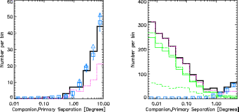
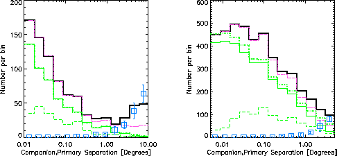
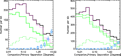
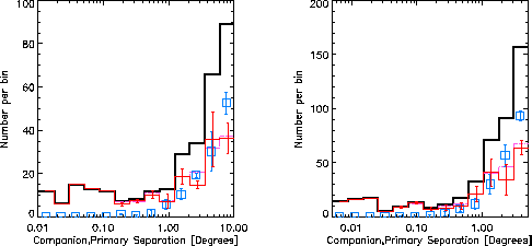
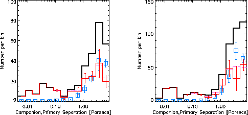
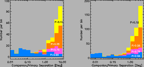
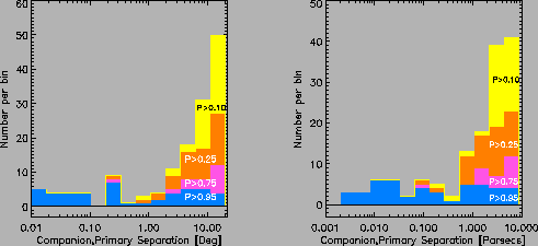
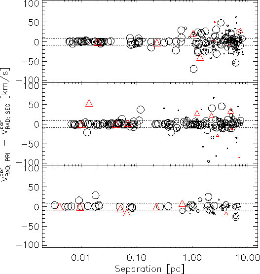
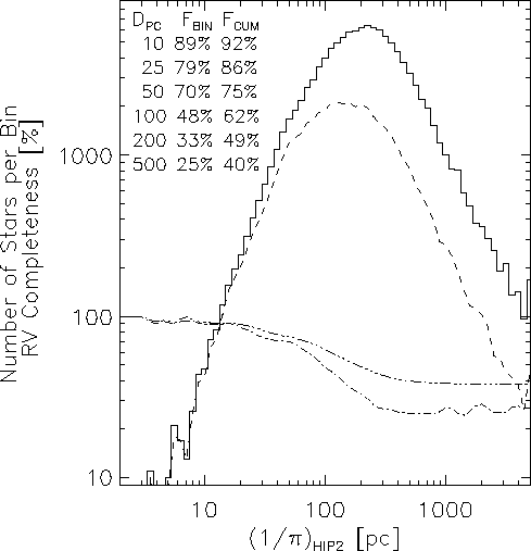
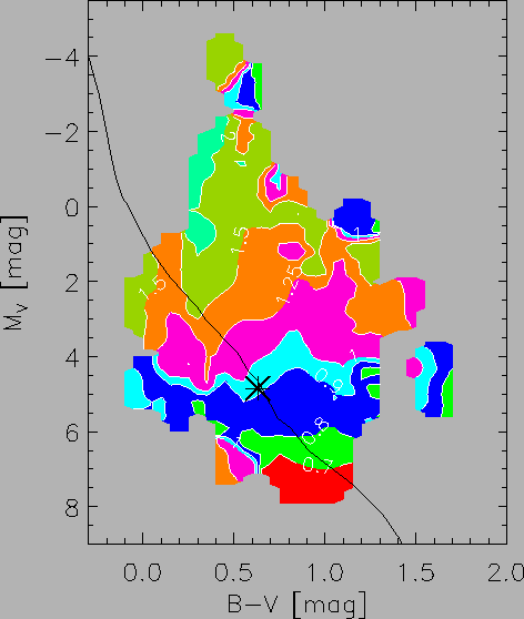 =1
contour, but at
=1
contour, but at  , indicates that the errors on the
inferred masses are not negligible: about 7.5% on the
MS, about 15% below the MS and up to 20% towards the top and
right-hand side of the map.
, indicates that the errors on the
inferred masses are not negligible: about 7.5% on the
MS, about 15% below the MS and up to 20% towards the top and
right-hand side of the map.
Tables
Table 1. Parameters for Probability Estimator| Distance |  |
 |
 |
 |
 |
 |
 |
 |
 |
 |
Nfmax | ||
| pc | |
|
|
pc | deg | deg | |
 |
|
|
|
||
| 0 – 25 | 35 | 45 | 100 | 20 | 0.01 | 20 | 10.0 | 0.97 | 7.13 | 0.97 | None | ||
| 25 – 50 | 25 | 35 | 75 | 15 | 0.01 | 10 | 3.44 | 0.93 | 3.39 | 0.78 | 12 | ||
| 50 – 100 | 10 | 20 | 50 | 20 | 0.005 | 5 | 2.09 | 1.06 | 2.28 | 1.15 | 10 |
Table 2. Attrition of Primary Stars
| Has | Nf | Has | # of Cs | # of Ps | Nc - | Nc - | ||||
| Distance | V<10 | Field | <Nfmax | Cs | P>0.1 | Pp>0.1 | Ncctrl | Ncctrl(<1pc) | Σ P | Σ P<1pc |
| 0 – 25 | 1041 | 786 | 786 | 369 | 144 | 111 | 84 | 34 | 85.7 | 26.9 |
| 25 – 50 | 4152 | 2916 | 2889 | 1119 | 316 | 265 | 194 | 89 | 198.7 | 72.5 |
| 50 – 100 | 14064 | 9018 | 8861 | 2090 | 504 | 464 | 258 | 99 | 301.3 | 106.5 |
| Total | 19257 | 12720 | 12536 | 3578 | 964 | 840 | 536 | 222 | 585.7 | 205.9 |
Note. –
Column 1 - distance interval of the row,
Column 2 - Number of stars brighter than V=10,
Column 3 - Number left after removing stars with no field stars or candidate companions,
Column 4 - Number left after removing those with too high field phase-space density,
Column 5 - Number left after removing those with no candidates,
Column 6 - Same as 5 but for separation < 1 pc only
Column 7 - Number of candidates with P>0.1,
Column 8 - Number of primaries with at least 1 candidate with
P>0.1,
Column 9 - Number of candidates - Number of candidates in
control experiments with P>0.1,
Column 10 - Σ P for candidates with P>0.1,
Column 11 - Σ P for candidates with P>0.1 and separated by less than 1 pc.