Next: About this document ...
ASTR615 Fall 2015 Problem Set #5
Due Wed November 18th, 2015
Write a program to integrate any number of coupled differential
equations using the Euler method, fourth-order Runge-Kutta, and
Leapfrog (note: Leapfrog only applies to special cases). You will be
using this program in a future assignment, so make sure it's well
documented. It's recommended that you use double precision
throughout.
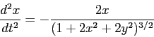
- Use your program to solve the following differential equation
for
 :
:
with initial conditions  ,
,
 . Note the
analytical solution is
. Note the
analytical solution is  .
.
- Integrate the equation for
 using each of the
methods, and step sizes of 1, 0.3, 0.1, 0.03, and 0.01.
using each of the
methods, and step sizes of 1, 0.3, 0.1, 0.03, and 0.01.
- Plot your integration results against the analytical solution
for each case. (Hint: do all the Euler plots on one page,
with one plot per timestep; then all the Leapfrog plots on another
page, etc.) Comment on the results.
- Plot
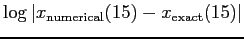 as a function of
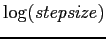 in each case and comment. (Hint: does the error have the
expected dependence on the stepsize? Remember you're integrating
over many steps, not just one.)
in each case and comment. (Hint: does the error have the
expected dependence on the stepsize? Remember you're integrating
over many steps, not just one.)
- Now try the two-dimensional orbit described by the potential:
where we are assuming unit mass for the particle in this potential.
Show analytically that the orbits are given by the coupled
differential equations:
and then reduce these to 4 coupled first-order equations.
- Integrate this system for
 with the initial
conditions
with the initial
conditions  ,
,  ,
,  ,
,  . Try
this with Leapfrog and Runge-Kutta, and step sizes of 1, 0.5,
0.25, and 0.1. Plot
. Try
this with Leapfrog and Runge-Kutta, and step sizes of 1, 0.5,
0.25, and 0.1. Plot  vs.
vs.  for these integrations.
- Plot the energy
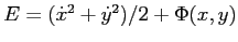 as
a function of time for your integrations.
as
a function of time for your integrations.
- Plot phase diagrams ( vs.
) for the Lotka-Volterra Predator-Prey model:
where is the prey density (rabbits), the predator density
(foxes),
 (rabbit reproduction rate),
  (rabbit
consumption rate by foxes),
(rabbit
consumption rate by foxes),  (fox death rate by natural
causes),
(fox death rate by natural
causes),  (fox population growth rate due to consumption
of rabbits), and
(fox population growth rate due to consumption
of rabbits), and  (hunting rate of foxes and rabbits,
respectively). Use only your Runge-Kutta integrator, with
(hunting rate of foxes and rabbits,
respectively). Use only your Runge-Kutta integrator, with  = 0
to 100 and timesteps of 1, 0.5, 0.25, and 0.1 to solve this system,
starting with
= 0
to 100 and timesteps of 1, 0.5, 0.25, and 0.1 to solve this system,
starting with  and
and  . If
. If  , for roughly
what value of
, for roughly
what value of  do both populations drop below
  by
by  for a timestep of 0.1?
Next: About this document ...
Massimo Ricotti
2015-11-18