- metadata:
various metadata is gathered from the input fits cube,
things like source name, vlsr, ra,dec,freq and their ranges and pixel sizes etc.
This is all gathered in XML files for later retrieval where needed.
- cubestats:
a (VO) table is produced with various statistics per plane
from the datacube. Most notably the Peak/Robust-RMS appears to be
a good indicator
of what spectral lines (at least the obvious ones) are in the dataset. The
strongest lines can easily be identified this way. I've used an
intensity weighted mean (some issues with the shape of the lines
are obvious).
- basic-map:
a simple sum (moment-0) of all the emission in the strongest line, just
getting an indication where the emission is. Again on the left the
extended array with higher resolution, on the right the compact array
with lower resolution. They nicely agree. A line is drawn accross
the emission which will be used in the next diagram.
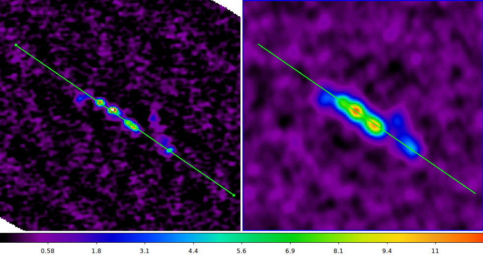
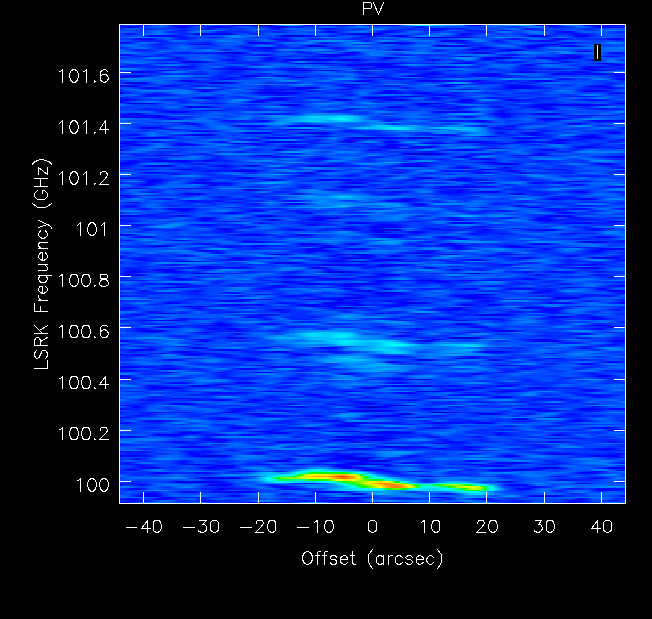
- Position-Velocity-Diagram (PVD) : a slice through the emission
is defined, and a PVD constructed from the cube.
You can clearly see a lot more
lines than in a typical spectrum (or Peak/RMS) diagram has seen before,
because of the coherent structures. This technique has been shown to
easily extend to 3D, but certainly in the compact array data made no
difference since no essentially new data is present off the slit.
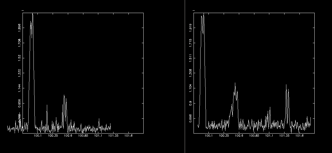
- PV Cross Correllation:
The strongest line from the cubestats output (hc3n)
will be used to calibrate the other weaker lines from. In theory
a few more can be used and a toothcomb fit could then be used.
Based on the RMS in the cube/map, an area around the strongest
line defines a template area which is then moved up and down and a
cross-correlation coefficient is computed. Below, on the left in red
is the cross-correlation,compared to the Peak/RMS plot we saw
earlier.
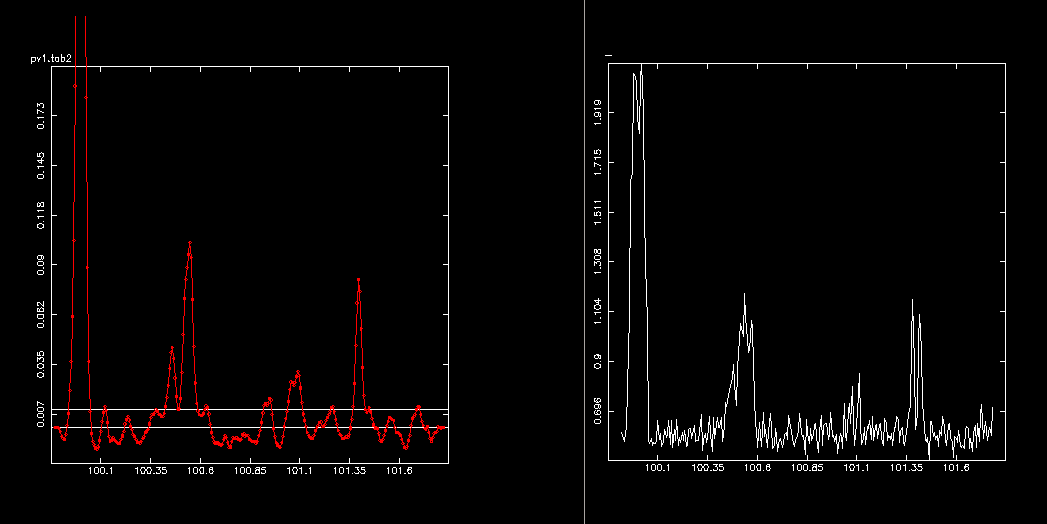
                                          Detection by traditional means:

101.477880 h2cs_1
101.139160 ch3sh
100.638900 ch3oh
100.076400 hc3n
                                          New and potentially new lines:
# SkyFreq   RestFreq    Corr
101.697941 101.778062 0.011628
101.449915 101.529840 0.010994
101.397464 101.477348 0.082473  h2cs_1
101.265428 101.345208 0.011990
101.090879 101.170522 0.031052  ?
101.060041 101.139659 0.025671  ch3sh
100.950088 101.029620 0.016209
100.927908 101.007422 0.013207
100.630415 100.709695 0.011976
100.547247 100.626461 0.102504  ch3oh
100.458107 100.537251 0.044464  ? nh2cn = cyanamide @ 100.51028
100.378348 100.457429 0.010009
100.120495 100.199373 0.011572
 99.997619 100.076400 1.000000  hc3n
There are at least 2 more lines visible in this spectral window that
had not been identified before, one is perhaps Cyanamide.
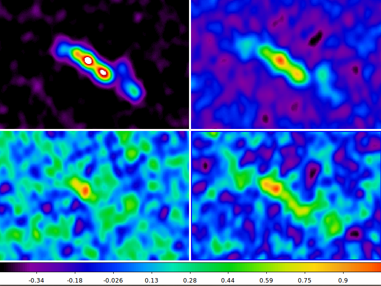
- Line Cubes:
Now that all lines have been identified, each line will get its own cube,
cut at the same doppler velocities instead of absolute sky frequencies,
so they can be compared. Shown here top to bottom, left to right, the
moment-0 maps of:
hc3n, ch3oh, ch3sh, h2cs_1.
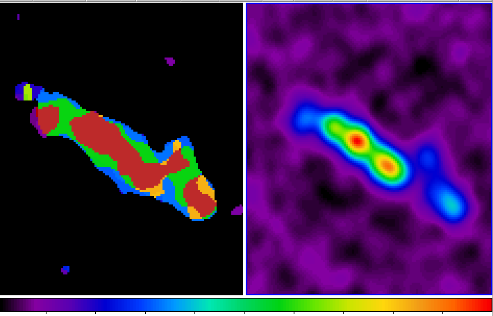
- Overlap Integral:
One interesting application is to see which lines are present
in which spatial parts of the map. We've constructed an overlap
integral map for this. In such a map the value
denotes (via a bit mask) which line is present at this location.
E.g. 255 means all 8 lines are present:
1 co     (adds 1 if present)
2 c17o   (adds 2
3 cn_1   (adds 4
4 cn_2   (adds 8
5 hc3n   (adds 16
6 ch3oh  (adds 32
7 h2cs_1 (adds 64
8 ch3c2h (adds 128
but for the value 191, you would see
1 co
2 c17o
3 cn_1
4 cn_2
5 hc3n
6 ch3oh
8 ch3c2h
thus only h2cs_1 is missing, since 191 = 255-64.
- clumpfind
HC3N:

Cl#  Xpeak   Ypeak   Vpeak         t0   FWHMx  FWHMy   R      FWHMv   Mlte        Err    Mgrav      N
----------------------------------------------------------------------------------------------------------------
  1    2.80    2.00  100.02   0.03     0.15    9.37    4.37    6.91    0.02  1.73E+02     1.0  1.95E-03    6657 A
  2   -4.40   -4.00   99.98   0.03     0.14    5.06    2.24    5.13    0.02  1.23E+02     1.0  1.30E-03    4172 A
  3  -16.00  -10.80   99.98   0.02     0.06    3.16    2.24    4.14    0.02  4.79E+01     1.0  9.88E-04    2619
  4  -11.20   -2.00   99.96   0.02     0.05    2.03    2.24    2.74    0.01  1.85E+01     1.0  1.64E-04    1012
  5  -11.20   -0.40   99.99   0.01     0.02    2.03    2.24    1.35    0.01  2.65E+00     1.0  7.08E-05     281 R
Total Mass: mlte= 0.3646E+03 mgrav= 0.4481E-02 Npixels=   14741


CH3OH:

Cl#  Xpeak   Ypeak   Vpeak         t0   FWHMx  FWHMy   R      FWHMv   Mlte        Err    Mgrav      N
----------------------------------------------------------------------------------------------------------------
  1   -4.80   -4.40  100.53   0.01     0.02    2.03    2.24    2.38    0.02  5.24E+00     1.0  2.84E-04     599
  2   -2.80   -3.20  100.51   0.01     0.01    2.03    2.24    2.54    0.02  3.11E+00     1.0  2.98E-04     433
  3  -11.60   -3.20  100.52   0.01     0.01    2.03    2.24    1.87    0.01  1.67E+00     1.0  4.32E-05     230 V
  4    2.40    1.20  100.55   0.01     0.01    7.64    2.24    3.81    0.02  4.55E+00     1.0  6.58E-04     654 A
  5    2.80    2.00  100.57   0.01     0.01    2.03    2.24    1.29    0.01  2.40E+00     1.0  8.63E-05     316
  6    6.80    4.80  100.58   0.01     0.01    2.03    2.24    1.09    0.01  8.36E-01     1.0  3.89E-05     112 R
Total Mass: mlte= 0.1780E+02 mgrav= 0.1409E-02 Npixels=    2344

CH3SH:

none found

H2CS_1:

Cl#  Xpeak   Ypeak   Vpeak         t0   FWHMx  FWHMy   R      FWHMv   Mlte        Err    Mgrav      N
----------------------------------------------------------------------------------------------------------------
  1   -4.40   -4.40  101.38   0.01     0.02    2.03    2.24    2.81    0.01  4.23E+00     1.0  1.49E-04     538
  2    3.20    2.00  101.42   0.01     0.01    8.41    2.24    4.32    0.01  6.65E+00     1.0  4.09E-04     936 A
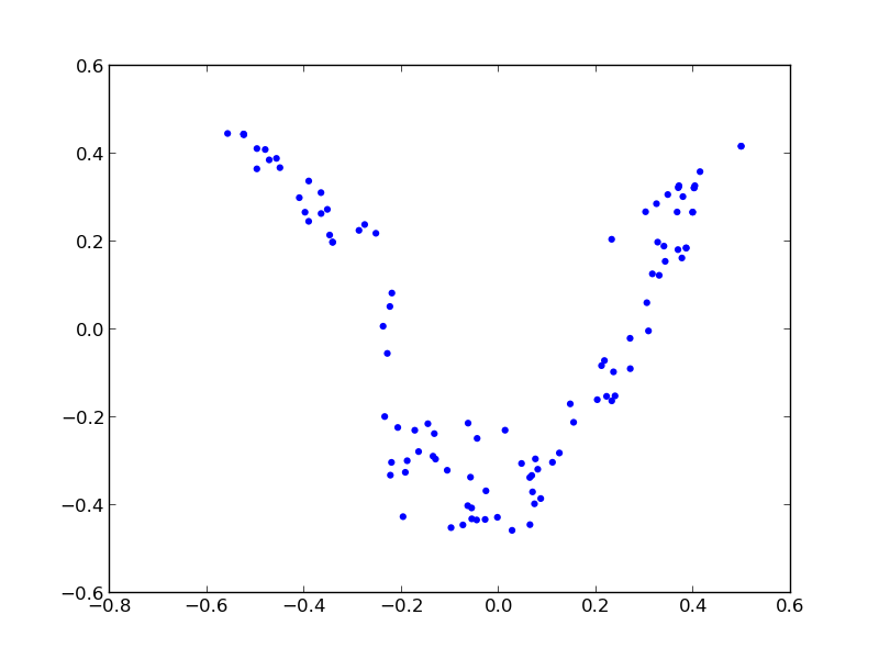
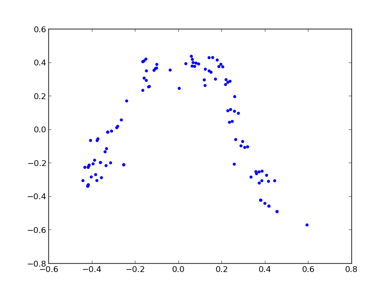
- Description Vectors
Make up properties of clumps, in this example the moments of inertia.
With an SVD compute centroids and shapes, "euler" angles, velocity
gradients (expansion or rotation) etc.