EFIDAD
Environment
For
Interactive
Data
Analysis and
Development
There are many valuable software tools available for interactive data analysis and development.
We made a selection of Python based tools and made them available on every machine. On this web page,
we present information about the installation status and list links to manuals on the web.
For a number of packages we provide examples. We invite you to contribute relevant examples.
A good tutorial which covers most of the tools described in the next table, is:
Using Python for Interactive Data Analysis by Perry Greenfield and Robert Jedrzejewski.
The base of the software listed in the next table is the current Python version on your system,
i.e. the version that is part of the RedHat Linux Enterprise destribution. For each package,
we list links to relevant documentation. Check for availability in the 'Installed' column of the table
below.
In one of the next sections we present some starters information and examples for most
of the listed packages.
The content of packages and modules can be viewed with
Pydoc
Overview of packages and their installation status
| Name | Purpose | Home page | Documents | Installed |
| python 2.3.4 |
 is an easy to learn, powerful programming language.
It has efficient high-level data structures and a simple but effective approach to
object-oriented programming. Python's elegant syntax and dynamic typing,
together with its interpreted nature, make it an ideal language for scripting and
rapid application development in many areas on most platforms. is an easy to learn, powerful programming language.
It has efficient high-level data structures and a simple but effective approach to
object-oriented programming. Python's elegant syntax and dynamic typing,
together with its interpreted nature, make it an ideal language for scripting and
rapid application development in many areas on most platforms.
|
Python home |
|
Yes |
| ipython |
Provide an interactive shell superior to Python's default.
IPython has many features for object introspection,
system shell access, and its own special command system for adding
functionality when working interactively. It tries to be a very
efficient environment both for Python code development and for exploration of
problems using Python objects (in situations like data analysis). |
Ipython home |
|
Yes |
| pyfits |
PyFITS provides an interface to
FITS
formatted files under the
Python
scripting language
|
Pyfits home |
|
Yes |
| numeric |
Numeric is an extension to the Python programming language, adding support for large,
multi-dimensional arrays and matrices, along with a large library of high-level
mathematical functions to operate on these arrays.
The original one, Numeric, which is reasonably complete and stable, remains available,
but is no longer supported.
|
Numeric download home |
|
Yes |
| numarray |
Numarray is an extension to the Python programming language, adding support for large,
multi-dimensional arrays and matrices, along with a large library of high-level
mathematical functions to operate on these arrays.
Numarray, is a complete rewrite of Numerical Python.
|
Numarray home |
|
Yes |
| matplotlib |
Matplotlib is a python 2D plotting library which produces publication quality figures
in a variety of hardcopy formats and interactive environments across platforms.
matplotlib can be used in python scripts, the python and ipython shell
(ala matlab or mathematica), web application servers, and six graphical user interface toolkits.
|
Maptplotlib home |
|
Yes |
| scipy |
SciPy is an open source library of scientific tools for Python.
SciPy supplements the popular Numeric module, gathering a variety of high level science and
engineering modules together as a single package.
SciPy includes modules for graphics and plotting, optimization, integration,
special functions, signal and image processing, genetic algorithms, ODE solvers, and others.
|
Scipy home |
|
Yes |
| scipy_core |
This package contains a powerful N-dimensional array object,
sophisticated (broadcasting) functions, tools for integrating C/C++ and Fortran code,
and useful linear algebra, Fourier transform, and random number capabilities.
It derives from the old Numeric code base and can be used as a replacement for Numeric.
It also adds the features introduced by numarray and can be used to replace numarray.
It is part of the latest 'scipy' version.
|
Scipy_core/Numpy home |
|
Yes |
| FFTW |
FFTW is a C subroutine library for computing the discrete Fourier transform (DFT)
in one or more dimensions, of arbitrary input size, and of both real and complex
data (as well as of even/odd data, i.e. the discrete cosine/sine transforms or DCT/DST).
|
FTTW home |
|
The C-lib is installed. Py. version follows |
| numdisplay |
Numdisplay provides the capability to visualize numarray array objects using astronomical
image display tools such as DS9 or XIMTOOL directly from the Python command line.
This task can display any numarray object, whether it was created interactively or read in
from a FITS file using PyFITS on any platform which supports Python and numarray.
This task has been developed by the Science Software Branch at the Space Telescope Science Institute.
|
Numdisplay home |
|
Yes |
| pyraf |
PyRAF is a new command language for running IRAF tasks that is based on the Python scripting language.
It gives users the ability to run IRAF tasks in an environment that has all the power
and flexibility of Python. PyRAF can be installed along with an existing IRAF installation;
users can then choose to run either PyRAF or the IRAF CL.
PyRAF is a product of the Astronomy Tools and Applications
Branch at the Space Telescope Science Institute.
|
PyRAF home |
|
Yes |
| MultiDrizzle |
MultiDrizzle automates and simplifies the detection of cosmic-rays
and the combination of dithered observations using the Python
scripting language and PyRAF, the Python-based interface to IRAF.
MultiDrizzle was developed by the Science Software Branch at the
Space Telescope Science Institute.
|
MultiDrizzle home |
|
YES |
| pyca |
PyCA (pronounced Pica, from itches in spanish)
is a Python module that computes Concentraction and Asymmetry of galaxies
using (preferentially) the by-products of SExtractor runs.
|
Pyca home |
|
No |
| pymidas |
PyMIDAS provides an interface from the Python scripting language to the ESO-MIDAS
astronomical data processing system.
It allows a user to exploit both the rich legacy of MIDAS software and the power of
Python scripting in a unified interactive environment which also opens up other
Python-based astronomical analysis systems such as PyRAF.
|
PyMIDAS home |
|
No |
| ParselTongue |
Python binding for classic AIPS
|
ParselTongue Home |
|
No |
| (py)gsl |
A python interface for the GNU scientific library (gsl).
The library provides a wide range of mathematical routines such as random number generators,
special functions and least-squares fitting. There are over 1000 functions in total.
|
PyGSL home |
|
Yes |
| gdl |
A free IDL (Interactive Data Language)
compatible incremental compiler (ie. runs IDL programs). Plots are based on plot package
plplot.
|
GDL - GNU Data Language
|
|
Yes |
| GNU Plotutils |
The GNU plotutils package contains software for both programmers and technical users.
Its centerpiece is libplot, a powerful C/C++ function library for exporting 2-D vector graphics
in many file formats, both vector and raster. It can also do vector graphics animations.
'libplot' is device-independent in the sense that its API (application programming interface)
does not depend on the type of graphics file to be exported.
Besides libplot, the package contains command-line programs for plotting scientific data.
Many of them use libplot to export graphics. Plotutils are used in the Biggles package. We did not
install a Plotutils Python binding.
|
Plotutils home |
|
Yes, the C library |
| gnuplot.py |
Gnuplot.py is a Python package that interfaces to gnuplot,
the popular open-source plotting program. It allows you to use gnuplot from within
Python to plot arrays of data from memory, data files, or mathematical functions.
If you use Python to perform computations or as `glue' for numerical programs,
you can use this package to plot data on the fly as they are computed.
And the combination with Python makes it is easy to automate things,
including to create crude `animations' by plotting different datasets one after another.
|
Gnuplot.py home |
|
Yes |
| biggles |
Biggles is a Python module for creating publication-quality
2D scientific plots.
|
Biggles home |
|
Yes |
| plplot |
The PLplot library can be used to create standard x-y plots,
semilog plots, log-log plots, contour plots, 3D surface plots,
mesh plots, bar charts and pie charts. Multiple graphs (of the same or different
sizes) may be placed on a single page with multiple lines in each graph.
A variety of output file devices such as Postscript, png, jpeg, LaTeX
and others, as well as interactive devices such as xwin, tk, xterm and
Tektronics devices are supported.
|
Plplot home |
|
Yes |
| PyX |
PyX is a Python package for the creation of PostScript and PDF files.
It combines an abstraction of the PostScript drawing model with
a TeX/LaTeX interface. Complex tasks like 2d and 3d plots in
publication-ready quality are built out of these primitives.
|
PyX home |
|
No |
| TableIO |
Reads/write ascii data from/to file
|
TableIO home |
|
No |
| pil |
The Python Imaging Library (PIL) adds image processing
capabilities to your Python interpreter. This library supports many file formats,
and provides powerful image processing and graphics capabilities.
|
PIL home |
|
Yes |
| ppgplot |
ppgplot is a python module (extension) providing bindings to the PGPLOT graphics library.
PGPLOT is a scientific visualization (graphics) library written in Fortran by T. J. Pearson.
|
ppgplot home |
|
No |
| vtk |
The Visualization ToolKit (VTK) is an open source, freely available software system for
3D computer graphics, image processing, and visualization used by thousands of
researchers and developers around the world.
|
VTK home
Using VTK Through Python
|
|
Yes |
| pyrex |
Pyrex lets you write code that mixes Python and C data types any way you want,
and compiles it into a C extension for Python.
|
Pyrex home |
|
Yes |
Help in Python and Ipython
| Python |
help([object])
|
Invokes the built-in help system.
No argument -> interactive help;
if object is a string (name of a module, function, class, method, keyword, or documentation topic),
a help page is printed on the console; otherwise a help page on object is generated.
|
| Python |
dir([object])
|
Without args, returns the list of names in the current local symbol table.
With a module, class or class instance object as arg, returns the list of names in its attr. dictionary.
|
| IPython |
?
|
Introduction to IPython's features.
|
| IPython |
%magic
|
Information about IPython's 'magic' % functions.
|
| IPython |
help
|
Python's own help system. Quit with q or ctrl-d
|
| IPython |
object?
|
Details about 'object'. ?object also works, ?? prints more
|
Information about modules and functions of packages that are installed on your computer
can be obtained via the EFIDAD
PYDOC server. The information about
the packages we are discussing, can be found in the section '/site-packages'.
For interactive mode type 'python' or 'ipython' on the Unix command line.
Scripts can be made in any editor. Python has its own integrated development environment.
It is called idle and is started with:
/usr/lib/python2.3/idlelib/idle
Browse the internet for tutotials for Python and IDLE.
Start with ipython on the command line. It will create an configuration file 'ipython'
in your home directory. You can log your commands if you start Ipython with: ipython -l.
Look in the man page, (man ipython) for more logging options.
An interesting combination is Ipython with interactive Matplotlib. In this mode, you
can give interactive plot commands and there is no need to draw the plot with the 'show()'
command. Here is a recipe (see also:
Using matplotlib interactively on the web):
Note that you may not want to update a plot every time a single property is changed if you
run a script, so keep a copy of your original 'matplotlibrc' file.
PyFITS provides functions to read FITS data. A two dimensional FITS image can be
displayed with the viewer DS9, using functions from module Numdisplay.
Example: numdisplay.example.1.py - Read image with pyfits and display with numdisplay
#! /usr/bin/env python

import pyfits
import numdisplay

pyfits.open('m101.fits')              # Open the fits file
im = pyfits.getdata('m101.fits')      # and read its data

numdisplay.open()  # If this doesn't work, start ds9 manually
numdisplay.display(im)
There a numerous plot packages for Python. One of
the oldest is the Python binding for Gnuplot. At the Kapteyn Institute we made Kplot/Kaplot as
a real object oriented alternative for Gnuplot. Now there is a package that is superior to
all other plot packages, and it is called Matplotlib. We strongly advise you to use this well
documented module for all your graphical output.
Example: matplotlib.example.1.py - The fastest way to get acquainted with Matplot
#! /usr/bin/env python
import pylab

x = pylab.arange(10)
y = x
pylab.plot(x,y)
pylab.show()
Example: matplotlib.example.2.py - Read x,y data from ascii file, plot and create PostScript file
#! /usr/bin/env python
import pylab

A = pylab.load( 'tgdata.dat', comments='!')
x= A[:,0]
y= A[:,1]
pylab.plot(x,y)
pylab.savefig( 'myplot.ps' )
pylab.show()
If you need to read data from a file with several columns and only want a range of lines, then
the function 'read_array' from the package 'scipy.io.array_import' in 'Scipy' is the better choice.
Scipy has its own help system. Here is an example how to use it on the Python command line:
>>>import scipy
>>>scipy.info(scipy.polyval)
Generates the text:
polyval(p, x)

Evaluate the polynomial p at x.  If x is a polynomial then composition.

Description:

  If p is of length N, this function returns the value:
  p[0]*(x**N-1) + p[1]*(x**N-2) + ... + p[N-2]*x + p[N-1]

  x can be a sequence and p(x) will be returned for all elements of x.
  or x can be another polynomial and the composite polynomial p(x) will be
  returned.

  Notice:  This can produce inaccurate results for polynomials with
  significant variability. Use carefully.
Example: scipy.example.1.py - Least squares fit with scipy's function 'leastsq'
#!/usr/bin/env python

from scipy import *
from scipy.optimize import leastsq
import scipy.io.array_import
import pylab

def residuals(p, y, x):
        err = y-peval(x,p)
        return err

def peval(x, p):
        return p[0]*(1-exp(-(p[2]*x)**p[4])) + p[1]*(1-exp(-(p[3]*(x))**p[5] ))

filename=('tgdata.dat')
data = scipy.io.array_import.read_array(filename)

x = data[:,0]
y = data[:,1]
pylab.plot( x, y , 'g.', linewidth='1')

# Initial guess of coefficients
A1_0 = 4
A2_0 = 3
k1_0 = 0.5
k2_0 = 0.04
n1_0 = 2
n2_0 = 1
p0 = array([A1_0 , A2_0, k1_0, k2_0,n1_0,n2_0])
yf = peval(x, p0)

#plot initial estimate
pylab.plot(x,yf, 'm')

plsq = leastsq(residuals, p0, args=(y, x), maxfev=2000)
p0_fit = plsq[0]

print plsq

# Plot function with fitted coefficients
yf = peval(x, p0_fit)
pylab.plot(x,yf,'r', linewidth='2')
pylab.show()
GDL is a free IDL (Interactive Data Language) compatible incremental compiler
(ie. runs IDL programs).
Start GDL with command gdl on the command line.
A simple plot is displayed with the following GDL commands:
GDL> orig = sin((findgen(200)/35)^2.5)
GDL> plot,orig
GDL> exit
You can configure GDL with a configuration file. First set an environment variable in your .cshrc
file:
setenv GDL_STARTUP /Users/users/yourname/.gdl_startup
Do not forget to source the file ( source .cshrc). An example of the content of this configuration file
called .gdl_startup
!PATH=!PATH + ':/usr/local/gdl/pro'
!PATH=!PATH + ':/Software/users/rsi/idl_6.0/lib/'
loadct,0, ncolor=255;
!P.BACKGROUND=255;
!P.COLOR=0;
!X.STYLE=1;
!Y.STYLE=1;
!Z.STYLE=1
print,'';
print, '*********************************************';
print, '** Personal settings are loaded and active **';
print, '*********************************************';
print,'';
Now you are able to load the .pro files located in the directories shown in the startup file.
Example: gdl.example.1.txt - Plot a fractal and also display a zoomed version.
GDL> appleman, RESULT=result
% Compiled module: APPLEMAN.
% LOADCT: Loading table BOW SPECIAL
GDL> window, 1
GDL> r=rebin(result,1280,1024)
GDL> tv,r[640:*,512:*]
GDL>
The Python binding has three methods only. These are:
- function(...) -- Execute a GDL function.
- pro(...) -- Execute a GDL procedure.
- script(...) -- Run a GDL script (sequence of commands).
Example: gdl.example.2.txt - GDL's Python binding
>>>import GDL
>>>print GDL.function("sin",(1,))
0.841470956802
The PyGSL documentation only describes the Python interface of routines that are
included in the GSL library. Suppose you want a program that generates random numbers
uniformly distributed in the range [0,1).
First have a look at the GSL Reference manual
which describes the C function that can do the job.
- Function: double gsl_rng_uniform (const gsl_rng * r)
- This function returns a double precision floating point number uniformly
distributed in the range [0,1). The range includes 0.0 but excludes 1.0.
The value is typically obtained by dividing the result of
gsl_rng_get(r) by gsl_rng_max(r) + 1.0 in double
precision. Some generators compute this ratio internally so that they
can provide floating point numbers with more than 32 bits of randomness
(the maximum number of bits that can be portably represented in a single
unsigned long int).
Now find the Python version of this function in the
Index of available functions
and you will find an item: rng (class in pygsl.rng)
Then the documentation shows the following information about this class:
This base class can be instantiated by its name

import pygsl.rng
my_ran0=pygsl.rng.ran0()
And the information about the uniform function is:
uniform() # returns a real number between [0,1).
So we expect the next Python code to work:
#! /usr/bin/env python

import pygsl.rng
x = pygsl.rng.uniform(10)
print x
But this does not work at all. If we ask Python to help ( start interactive session, import
pygsl.rng and type help(pygsl.rng))
Then you will find that the distribution is called 'uni' and not 'uniform'.
The constructor (pygsl.rng.uni()) also does not allow a number to initialize. Instead we need to
create an array (y) which generates 10 random numbers using the new object (x).
#! /usr/bin/env python

import pygsl.rng
x = pygsl.rng.uni()
y = x(10)
print y
Example: pygsl.example.1.py - Fit a function to noisy data and plot the result
#! /usr/bin/env python

import pygsl
import pygsl._numobj as Numeric
import pygsl.rng
import pygsl.multifit
import pylab


def calculate(x, y, sigma):
    n = len(x)
    X = Numeric.ones((n,3), Numeric.Float)
    X[:,0] = 1.0
    X[:,1] = x
    X[:,2] = x ** 2
    w = 1.0 / sigma ** 2
    work = pygsl.multifit.linear_workspace(n,3)
    c, cov, chisq = pygsl.multifit.wlinear(X, w, y, work)
    c, cov, chisq = pygsl.multifit.linear(X, y, work)


    print "# best fit: Y = %g + %g * X + %g * X ** 2" % tuple(c)
    print "# covariance matrix #"
    print "[[ %+.5e, %+.5e, %+.5e ] " % tuple(cov[0,:])
    print " [ %+.5e, %+.5e, %+.5e ] " % tuple(cov[1,:])
    print " [ %+.5e, %+.5e, %+.5e ]]" % tuple(cov[2,:])
    print "# chisq  = %g " % chisq
    return c, cov, chisq

def generate_data():
    r = pygsl.rng.mt19937()
    a = Numeric.arange(20) / 10.# + .1
    y0 = Numeric.exp(a)
    sigma = 0.1 * y0
    dy = Numeric.array(map(r.gaussian, sigma))
    return a, y0+dy,  sigma


x, y, sigma = generate_data()
c, cov , chisq = calculate(x, y, sigma)
pylab.plot(x,y)
xref = Numeric.arange(100) / 50.
yref = c[0] + c[1] * xref + c[2] * xref **2
pylab.plot(xref,yref)
pylab.show()
Biggles needs to access a library in the directory /usr/local/lib. To add this path to
your standard library path, add the following line to your .cshrc file in your home directory
and type source .cshrc afterwards.
setenv LD_LIBRARY_PATH ${LD_LIBRARY_PATH}:/usr/local/lib
Example: biggles.example.1.py - Simple plot with Biggles, output is a plot in png and PostScript format
#! /usr/bin/env python

import biggles
import Numeric, math

x = Numeric.arange( 0, 3*math.pi, math.pi/30 )
c = Numeric.cos(x)
s = Numeric.sin(x)

p = biggles.FramedPlot()
p.title = "title"
p.xlabel = r"$x$"
p.ylabel = r"$\Theta$"

p.add( biggles.FillBetween(x, c, x, s) )
p.add( biggles.Curve(x, c, color="red") )
p.add( biggles.Curve(x, s, color="blue") )

p.write_img( 400, 400, "example1.png" )
p.write_eps( "example1.eps" )
p.show()
In the Plplot example below, the application prompts for a device. Enter either a number or
a name from the list that is displayed. The example can be aborted by closing the plot window.
Example: plplot.example.1.py - Simple plot with Plplot
#! /usr/bin/env python

import plplot

plplot.plsdev( plplot.plgdev() )
plplot.plinit()
plplot.plcol0( 3 )

plplot.plenv (-0.5, 5, -0.5, 5, 0, 0)
x = (0,1,2,3,4,5)
y = (1,3,5,3,5,1)

plplot.plline (x, y)
plplot.plend ()
Gnuplot can be used in two modes. First you can import the Gnuplot package and use its functions
directly. You find an example in gnuplot.example.1.py
In the other method we use the popen package included in the os module.
With popen it is possible connect to the stdin (or stdout) of a program through a pipe.
The code below (data in xrddata.dat) more or less shows how example 1 is reproduced
using popen instead of the gplt package. The major difference is the fact that
with popen it is not necessary to import the data to be plotted into
Python - instead it is read directly by gnuplot.
Example: gnuplot.example.2.py - Access Gnuplot with 'popen'
import os

DATAFILE='xrddata.dat'
PLOTFILE='xrddata.png'
LOWER=35
UPPER=36.5

f=os.popen('gnuplot' ,'w')
print >>f, "set xrange [%f:%f]" % (LOWER,UPPER)
print >>f, "set xlabel 'Diffraction angle'; set ylabel 'Counts [a.u.]'"
print >>f, "plot '%s' using 1:2:(sqrt($2)) with errorbars title 'XRPD data' lw 3" % DATAFILE
print >>f, "set terminal png large transparent size 600,400; set out '%s'" % PLOTFILE
print >>f, "pause 2; replot"
f.flush()
Python examples for VTK can be found on the
vtk Python examples page.
In these examples you find references to a data area. Replace these references to a local copy of
this data on our fileserver in the directory:
/Software/users/VTK/VTKData/
Example: pil.example.1.py - Use PIL functions to display an image
#! /usr/bin/env python

import Image
im = Image.open("foto1.jpg")
im.show()
Suppose you write a script that opens a fits file and wants to clip its data with
some value. If the name of the file and the clip level are variables, then it is
more flexible to read these values from the command line when you execute the script.
The command line arguments are read as strings. So the clip level has to be
casted to a floating point number. You need module 'sys' to import the functionality
to read command line arguments. In this script you will get a usage message if you do not
enter 2 command line arguments. Note that if your clip level cannot be converted to
a floating point number, an exception will be raised. In the second example we show how
to process such an exception.
Example: python.example.1.py - A script that expects 2 command line arguments
#!/usr/bin/python

from sys import argv

if len(argv)!=3:
    print "Usage:", argv[0],"  "
    raise SystemExit

print "Name of this script=", argv[0]
print "Fits file name = ", argv[1]
print "Clip level = ", float(argv[2])
If you have applications written in C or Fortran, or want to use system commands, and you
need to process the output of these programs in your Python script, then there is an
easy way to do this with function 'popen'. In the next example, the script is a 'big file' finder.
It reads file names in the current directory and its sub directories.
When the size of a file is greater than 1000k, the name is printed.
The Unix command 'ls' is used to generate the list, which is read by the function 'popen'.
The Python code uses 'readlines' to process the 'ls' output line by line.
There are two complications in the script. First we have to remove the new line
character at the end of strings that are read by the 'readline' function.
The second complication is that sometimes a string does not represent a number followed by a name.
Then the conversion to an integer fails and an exeption is raised. In the next example
we handle the exception by setting the involved variable to 0.
Example: python.example.2.py - Using 'popen' to read the results of a system call
#!/usr/bin/python

import os, string

filenames = os.popen('ls -Rsk', 'r' )           # Communicate with external process
while (1):
   f = filenames.readline()
   if f:
      fclean = f.rstrip()                       # Remove the newline character
      parts = fclean.split( ' ' )
      if (len(parts) == 2):                     # Continue if we have 2 strings
         (s, name) = parts                      # Copy splitted str in 2 variables
         try:                                   # Not all strings can be converted to int
            si = int(s)
         except:
            si = 0
         if (si > 1000):
            print "BIG: %s is %d k" % (name,si)
   else:
      break
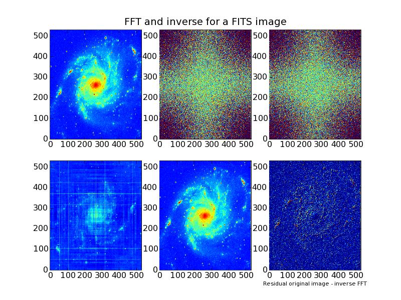
Below the output of a small program that reads image data from a FITS file.
It transforms the image using an FFT from package FFT2 (or in fact fftw).
The plot shows the original image, the real part and the imaginary part of
the transform. Finally the inverse transform results in again two images.
A real part which should be equal to the original image and a imaginary part.
The last subplot is the residual and shows the quality of the FFT.
Note that for the functions we used to calculate the inverse FFT, it is not needed to
scale the result. Therefore the residual is simple the difference between the
original image and the real part of the inverse FFT.
It is important to note that the matrices from 'pyfits' are numarray arrays.
The matrices that are a result of the MLab rot90 function however are Numeric arrays.
You cannot subtract them without converting one to the type of the other.
Example: fftw.example.1.py - Use module FFT2 (fftw) to transform an image
#! /usr/bin/env python
import pyfits
import sys,types,FFT2
import numarray, Numeric
import pylab, MLab

file  = sys.argv[1]                             # Argument on command is FITS file
hdr   = pyfits.open( file )                     # Open the FITS file for reading the data
print hdr.info()                                # Show top level header info
naxis = hdr[0].header['naxis']                  # Get the number of axes in the image
print 'Number of axes in this image = %d ' % (naxis)

img = hdr[0].data                               # Get image data
print "Dimensions of image data = %s.  Type of data is: %s" % (img.shape, img.type())
if (naxis == 2):
   pylab.subplot( 231 )
   pylab.imshow( img, vmin=img.min(), vmax=img.max() )
   (l,m) = img.shape
   mi    = img.min()
   ma    = img.max()
else:                                           # Not 2dim, no use to continue
   sys.exit()

C = FFT2.fft2d( img )                           # FFT this image
pylab.subplot( 232 )                            # Plot real and imaginary parts
pylab.title('FFT and inverse for a FITS image')
pylab.imshow( C.real, vmin=-100000.0, vmax=100000.0 )
pylab.subplot(233)
pylab.imshow( C.imag, vmin=-100000.0, vmax=100000.0  )

D = FFT2.ifft2d( C, C.shape )                   # Calculate inverse
pylab.subplot( 234 )
pylab.imshow( D.imag )

InvFFTrot = MLab.rot90( D.real, 2 )             # Inverse was rotated 180 deg.
pylab.subplot( 235 )
pylab.imshow( InvFFTrot )

# Calculate the residual bu subtracting two matrices
# which has their origin from different numerical packages
# cast the image (from numarray) to the type of array
# InvFFTrot (Numeric)

diff = InvFFTrot - Numeric.array( img )         # Calculate residual.
pylab.subplot(236)
pylab.imshow( diff, vmin=mi/10., vmax=ma/10. )
pylab.xlabel('Residual original image - inverse FFT', fontsize=8 );

hdr.close()                                     # Close FITS file
pylab.show()                                    # Show the plot
There are several methods to read data from an ASCII file. The simplest is the built-in Python function
readlines. For more advanced io for ASCII tables, you should read the documentation of the module
io.array_import form Scipy.
The documentation of its functions is in Pydoc format and can be found in
scipy.io.array_import.
Assume you have a plain text file with two columns of data. There are no comment lines
and you want to read all the data into two arrays. The next example shows how to read these lines.
Example: scipy.io.example.1.py - Read data from an ASCII file
#!/usr/bin/env python
import scipy.io.array_import

filename=('tgdata.dat')
data = scipy.io.array_import.read_array( filename )

x = data[:,0]
y = data[:,1]
Have a look at the contents of some ASCII file with data:
name    s1      s2      s3      s4
Jane    98.3    94.2    95.3    91.3
Jon     47.2    49.1    54.2    34.7
Jim     84.2    85.3    94.1    76.4
If we want to extract the array containing just the numbers, use the columns
and lines arguments. Note that the first column corresponds to index '0'.
>>> a = io.array_import.read_array('a.dat',columns=(1,-1), lines=(1,-1))
>>> print a
[[ 98.3  94.2  95.3  91.3]
 [ 47.2  49.1  54.2  34.7]
 [ 84.2  85.3  94.1  76.4]]
If you want to create a matrix with second and third column only, you have to change the
columns argument to: columns=(1,2)
>>> a = io.array_import.read_array('a.dat',columns=(1,2), lines=(1,-1))
>>> print a
[[ 98.3  94.2]
 [ 47.2  49.1]
 [ 84.2  85.3]]
A more practical example is extracting three columns 'x', 'y' and 'z' from
the data, which should contain columns 1 to 3 (i.e. 1, 2) and 4 of all lines in the file.
Note that when a tuple is part of the columns argument, then this tuple defines a range of columns.
>>> data = io.array_import.read_array('a.dat',columns=((1,3),4), lines=(1,-1) )
>>> x = data[:,0]
>>> y = data[:,1]
>>> z = data[:,2]
>>> print x, y, z
[ 98.3  47.2  84.2] [ 94.2  49.1  85.3] [ 91.3  34.7  76.4]
Suppose the first character of the third line was '#' and
this character indicates that
the line should be ignored (content is wrong or is a comment),
then we have to set the argument for the comment character.
>>> data = io.array_import.read_array('a.dat',columns=((1,3),4), lines=(1,-1), comment='#' )
>>> x = data[:,0]
>>> print x
[ 98.3  84.2]
If you want to read your data as another type than the default (float), then you should
give a so called typecode. If the numbers in the file are complex numbers, then the typecode
is 'D'. The contents of the modified ASCII file is now:
name    s1           s2      s3      s4
Jane    98.3         94.2    95.3    91.3
#Jon    47.2         49.1    54.2    34.7
Jim     84.2+2.2j    85.3    94.1    76.4
Then the trick to read the numbers as complex numbers is:
>>> data = io.array_import.read_array('a.dat',
           columns=((1,3),4), lines=(1,-1), comment='#', atype='D' )
>>> x = data[:,0]
>>> print x
>>> [ 98.3+0.j   84.2+2.2j]
If a column has a complex number but the typecode is not complex, then a warning is raised
with message "Warning: Complex data detected, but no requested typecode was complex",
However, the data is read in the requested format. Note that you can also give a tuple of
typecodes (like: atype=('d','D')). The result is two arrays, one of type 'd' and one of type 'D'.
Below a list with type codes and aliases for numarray numbers:
Int8         '1', "i1", "Byte"
Int16        's', "i2", "Short"
Int32        'i', "i4", "Int"
UInt8        "u1", "UByte"
UInt16       "u2", "UShort"
Float32      'f', "f4", "Float"
Float64      'd', "f8", "Double"
Complex64    'F', "c8", "Complex"
Complex128   'D', "c16"
The output of the 'read_array' method can be seen as an array of lines.
Therefore you cannot (unless you transpose the matrix)use
a syntax like
(x,y,z) = io.array_import.read_array('a.dat',
          columns=((1,3),4), lines=(1,-1), comment='#', atype='D' )
to read your columns. You have to set your columns to the right data slice with:
>>> x = data[:,0]
>>> y = data[:,1]
>>> z = data[:,2]
If you prefer to read the data directly in columns, you first have to transpose the matrix
that contains the data read from file. Here is an example:
(x,y,z) = scipy.transpose(io.array_import.read_array('a.dat',
          columns=((1,3),4), lines=(1,-1), comment='#', atype='D' ))
>>> print x
[ 98.3+0.j , 84.2+2.2j,]
>>> print z
[ 91.3+0.j, 76.4+0.j,]
Finally a simple example how to write a matrix to an ASCII file ('data.dat'.
We generated an array
of 100 floating point numbers. The array is converted to a matrix with 20 rows and
5 columns. The write_array function accepts the name of a file (or a file pointer),
and writes the data to a plain text file. We set the column separator to a comma
followed by a space to create a file in 'Comma Separated Format' (easy to import in
a spreadsheet). The example also shows how to set the precision of the floating point
numbers in the file. The function closes the file after the function call. To prevent
this automatic closing of the file on disk, use function argument 'keep_open' with
a non-zero value.
Example: scipy.io.example.2.py - Write array data to ASCII file
#!/usr/bin/env python

import scipy
import scipy.io.array_import

mydata = scipy.arange(100.0)   # Generate 100 floating point numbers
mydata.shape = (20,5)          # 20 rows, 5 columns

scipy.io.array_import.write_array( 'data.dat', mydata, separator=', ', precision=1 )