N rigid-body dynamics

SHORTCUTS: Reading Notes Homework

PiTP 2009 Richardson Lecture: Suggested Reading

My lecture will be a short introduction to the N-body problem augmented by rigid body motions, including collisions. Simulations of this sort are applicable to planet formation (planetesimal/asteroid/comet evolution), planetary ring dynamics, and granular dynamics in general.

A basic understanding of how to solve ordinary differential equations numerically will be assumed. Good background reading includes the "Integration of Ordinary Differential Equations" chapter of Numerical Recipes (any edition), particularly the introduction and the section on the Runge-Kutta method.

Good sources on the N-body method in general are scarce, but if you have access to the 2008 edition of Lecture Notes in Physics, Volume 760, there is a chapter in there by Sverre Aarseth entitled "Direct N-body Codes" that would be worthwhile to read. Also, Barnes & Hut's 1986 Nature paper on tree codes would be useful.

Appendix D.2 of the second edition of Galactic Dynamics (Binney & Tremaine) gives some background on systems of particles and rigid bodies in general. For the particular approach I will use in my lecture, including the collisional physics, you can skim my paper Numerical simulations of asteroids modelled as gravitational aggregates with cohesion.

As an exercise, we will be using the N-body code I helped develop, pkdgrav, to carry out a small simulation of self-gravitating, rigid body mechanics. Unfortunately this version of the code is not in the public domain (yet).

PiTP 2009 Richardson Lecture: Lecture Notes

The notes from my lecture are available as a PDF. I showed a lot of movies in my talk. If you're interested in obtaining any of these, please e-mail me: dcr (put @ symbol here) astro.umd.edu.

PiTP 2009 Richardson Lecture: Exercise

If you would like to play around with pkdgrav a bit, try the following exercise:

1. If you have a copy of ss_core.tar.gz, unpack it, run "build" in the directory that is created, and choose option 3 for aggregates (otherwise select defaults). If you don't have the source code (that's most of you), log in to the apollo cluster (remember to "qsh" right away), then "astroload pkdgrav".
2. Create a run directory (call it whatever you like), cd to it, and copy the following files into it: rpg.par, ss.par, ssdraw.par, world.ss.
3. Execute "pkdgrav +overwrite ss.par" (optionally redirecting stdout to a file). If all goes well, a bunch of output files should be generated.
4. Create a movie of the result by executing "mkmov". View the resulting movie.mpg using your favorite movie player. Here's what you should get: movie.mpg. (Yes, it takes longer to make the movie than to run the simulation!)

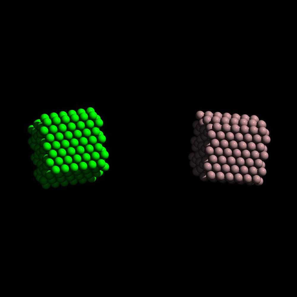
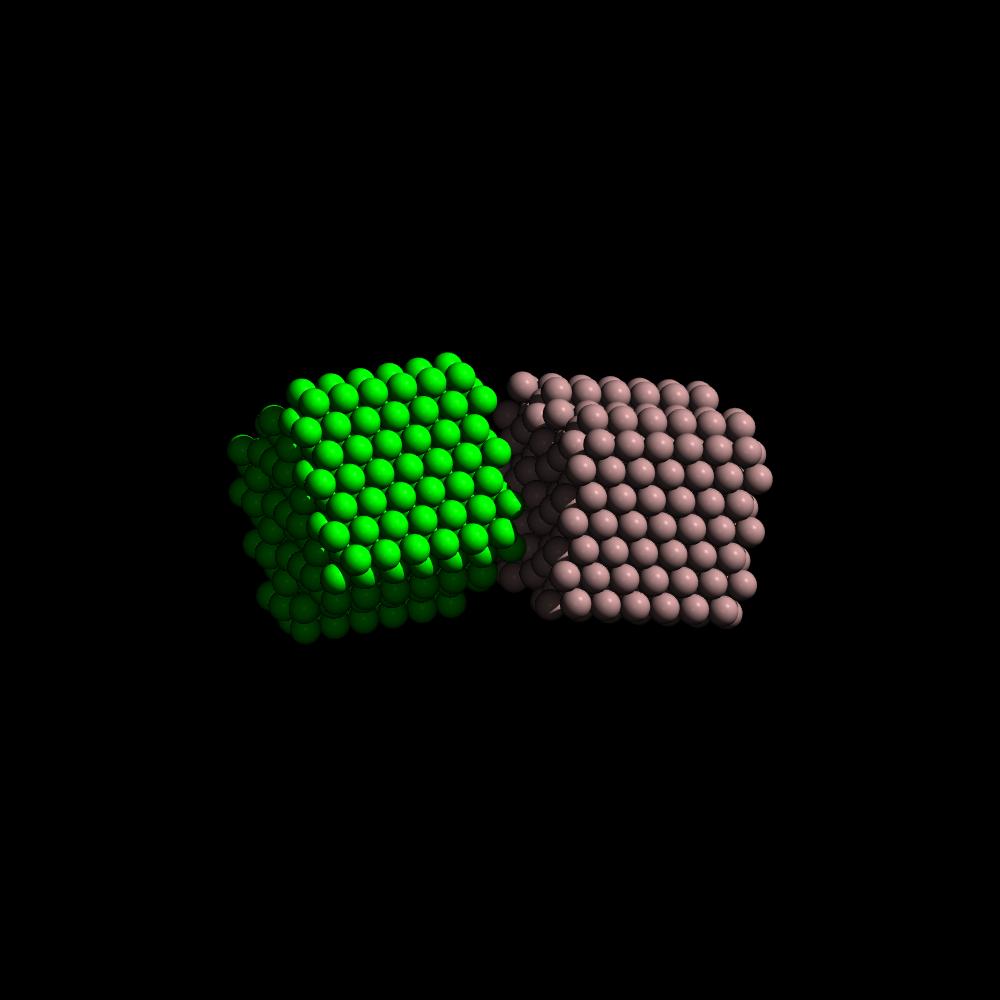
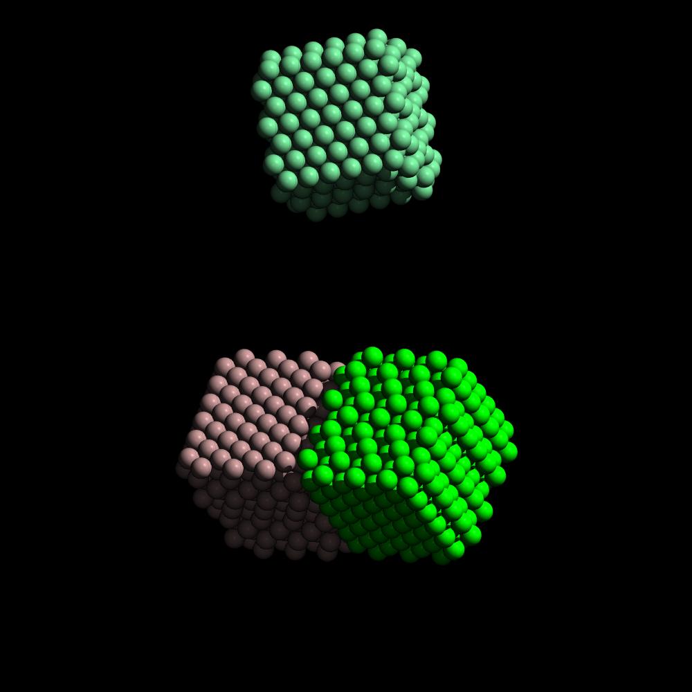
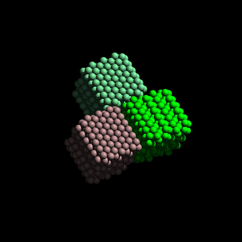
So what did you just do? This was a simulation of two weak km-size bonded aggregates (asteroids) that collide at 10 m/s. If you want to try your own scenario, you need to know how to generate initial conditions and choose reasonable simulation parameters. Here are some tips:

1. The utility "rpg" generates rubble piles according to the parameters in rpg.par. Feel free to tweak the basic parameters like axis lengths, bulk density (what would changing the bulk density do?), number of particles, spin, and whether the rubble pile should be tagged as a bonded aggregate (give it a unique aggregate ID >= 0). This creates rpg.ss. Use the utility "rpx" to adjust and combine one or more rubble piles into a single file (I used "world.ss") -- you can set up the piles so they smash into each other or whatever. HINT: say "N" when asked if you want to use simulation units -- it will be easier.
2. Alternatively, generate your own initial conditions by hand. To do this, you need to understand the data format. An "ss" file is binary, but you can create a human-readable intermediary "bt" file with the following format: one particle per line, with each line consisting of: idx orgidx m R x y z vx vy vz wx wy wz color, where: idx is an integer that should be 0 for the first particle, 1 for the second, etc.; orgidx is an integer that should be either equal to idx, or, if you want to make the particle part of an aggregate, a negative number indicating the aggregate ID (= -1 - orgidx); m is the particle mass; R is the particle radius; x, y, z are the particle position components; vx, vy, vz are the velocity components; wx, wy, wz are the spin components; and color is an integer (1=white, 2=red, 3=green, 4=blue; see the end of ssdraw.par for the key). Units: G=1. So a standard system is masses in solar masses, lengths in AU, and time in yr/2pi (so speeds are 2pi AU/yr, i.e. ~30 km/s, the mean speed of the Earth around the Sun). When you're done, convert the file to ss format using "bt2ss".
3. pkdgrav reads the run parameters from ss.par. The ones to play with are dDelta (time step), nSteps, achInFile (initial conditions file name), iOutInterval (output interval; iRedOutInterval controls "reduced" output files more suitable for movie making than analysis), bVStep (set it to 0 to reduce verbiage), iOutcomes (a bit field that dictates what collision outcomes are allowed, e.g. 7 = 1 + 2 + 4 means merging/sticking, bouncing, and fragmentation are all allowed), dMergeLimit (impact speeds less than this result in sticking---note the comment about the units), dEpsN and dEpsT (bounce coefficients), and dFragLimit (impact speeds greater than this result in breaking). There are plenty of other parameters of course...feel free to experiment, but your mileage may vary!
4. IMPORTANT: for a sensible simulation, your run parameters and initial conditions need to be consistent. For example, the timestep should reflect the shortest dynamical scales you expect in the problem. Most new simulations require a few back-of-the-envelope calculations to set things up correctly.
5. Visualization parameters are in ssdraw.par. Run "ssdraw" on any ss file to create a graphical image (rasterfile) that can be viewed with a utility like "xv". Or use the "mkmov" script to generate a movie from all output files in the run directory. If you're familiar with POV-Ray, ssdraw can create output files suitable for this ray tracer---see me if you want to try this.
6. For simple analysis, try running rpa on your output files (e.g. "rpa ss.?????"). If you have the plotting package sm, grab rpa.sm and try "sm inp_new rpa.sm".
7. Have fun!