Chapter 1
There is a lot of purple prose out there about astronomy. Education and Outreach professionals and amateurs alike are basically dying to excite others as much as they are excited themselves. Sometimes that excitement is totally justified, but we run the risk of creating two models of the universe in your head: one for "real life" on a day to day basis and one that only seems to exist in splashy Discovery Channel specials or worse, only in the classroom. Neil deGrasse Tyson gets it right in the video link here. You should live your life in awe at least once a day and you should take what you learn in this astronomy class (and others) to heart every time you look up at the sky.
We begin our tour. For more info on the Messenger mission to Mercury: click here.
For cool fly-over movies of Venus based on real data, check out David P. Anderson's website at SMU. Cutting edge computer animation for its time. Still looks cool, even in the age of Pixar.
The order of the planets if you haven't already memorized it: "My Very Eccentric Mother Just Showed Us Nine Planets." Well, Pluto is now just a dwarf planet along with thousands of other KBOs. So, instead, maybe you should learn, "My Very Eccentric Mother Just Served Us Nachos." Meh.
And then there are the seven moons worth remembering: our Moon, Io, Europa, Ganymede, Callisto, Titan and Triton. Do you know which planets they each go around? (Earth, Jupiter, Jupiter, Jupiter, Jupiter, Saturn and Neptune.) What does it take to be a decent size? Look at figure 1.16 in the book. Any smaller than 200 km in diameter, and your object isn't likely to be spherical. CAREFUL HERE: there are loads of objects/moons/etc. larger than 200 km in size, NOT just seven...
Maxwell Montes, Venus
David P. Anderson, SMU Geophysics
Here's the link to the moon movie I showed in class, which gives you a quick sense of how different the near and far sides of the moon are.
Don't forget to visit Google Mars!
This is an even better movie of the strange white storm on Saturn. This was in Saturn's Northern Summer of 1991. Quick: When's the next one coming? (Look up Saturn's orbital year and add that to 1991).
Here is a great collection of carefully reconstructed images of Titan from real data!
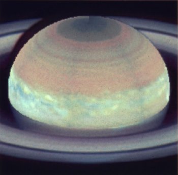
The Great White Spot
(shmeared in this Hubble photo)
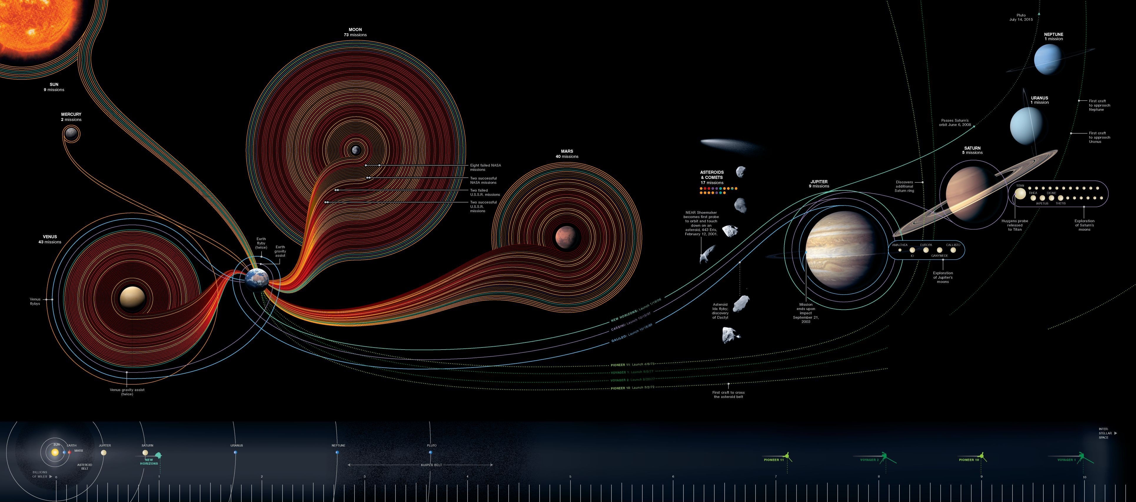
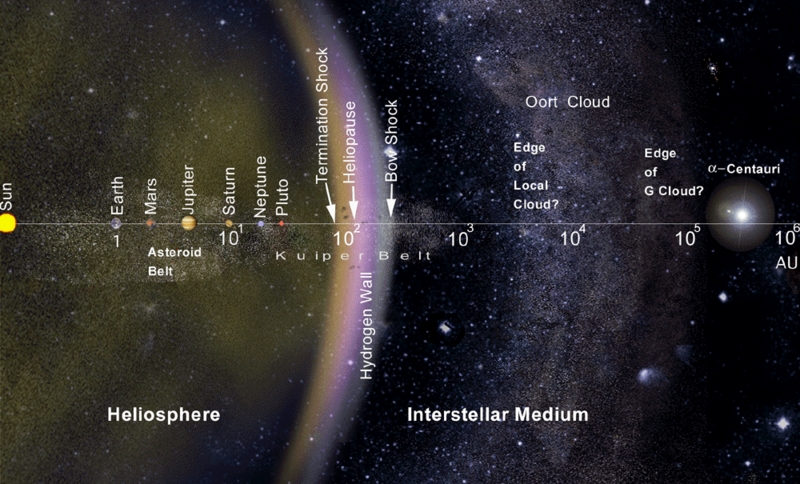
Check out this cool graphic regarding the scales of the solar system, but BEWARE! The scale from left to right is logarithmic in AU. That is, equal intervals represent an increase in ten times the previous distance. Contemplate this picture again when we've reviewed logarithms.
Chapter 2 & 3
If anyone is ever going to drill through the Moho boundary, it'll be some group connected to the International Oceanic Drilling Project.
You'll note the dates on these articles: still, six+ years later, no one has "poked" through the Moho discontinuity.
We had a little taste of California shakin' in August 2011. Here's a great video showing the P and S waves as they disperse through the North American plate. Note the speed difference, too.
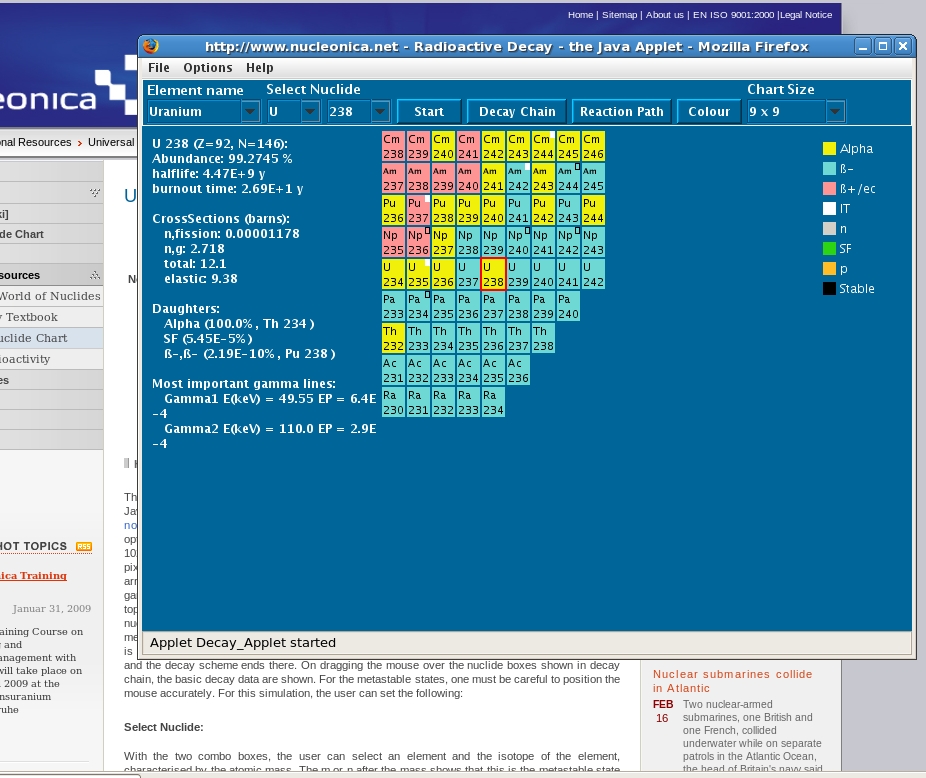
Here's a way to see where things "go" when they decay away. You can note, for instance, that 26Al isn't actually gone. It's just hiding as 26Mg instead! Click on the big, gray "Universal Nuclide Chart" button. Then choose your element (e.g., Al) and choose your isotope (26) and hit "Decay Chain." Pretty dull, eh? Okay, now try Uranium (U) 238 or 235. Now that's decay for you! If you hover with the mouse over each box, it displays the half-life for that isotope.
Here is a pdf of some of the class slides.
For the record, the list of bonds really was in (very rough) strength order; that is from strongest to weakest (as a rule, but not a hard and fast one!) metallic, ionic, covalent, molecular. Some metals have easy bonds to break/low melting points (think Hg = Mercury); some covalent bonds are fairly strong. What I want you to take home from all this confusion is that when something is refractory, it doesn't melt at low temperatures, i.e., the bonds (whichever kind) are relatively strong. When something is volatile, it's the opposite situation. The bonds that form water ice (melting point 0 oC = 273 K) are not as strong as those that hold silicon dioxide (quartz, melting point 1650 oC = 1923 K) or chunks of iron (melting point 1535 oC = 1808 K) or carbon (sublimation around 3600 oC ~ 3900 K). This oversimplified picture is ignoring actual chemical reactions (like combustion, or corrosion) which generally drive things towards ever-stronger types of bonds.
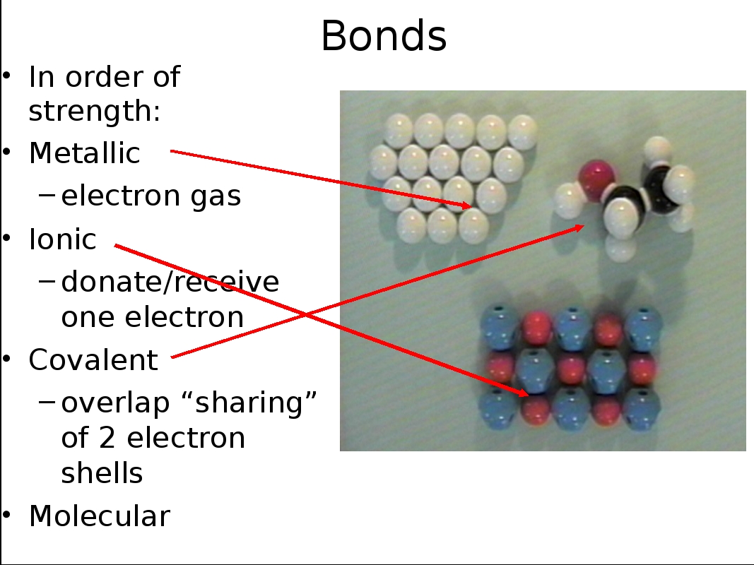
Plate tectonics in a very cool animation.
Also, here is an article from September 2011 Science magazine which points out that Mercury may not be as "weird" as we think. Messenger is finally deciphering what Mercury might be made of and the degree of differentiation at the surface, a.k.a., the crust, tells us a lot about Mercury's origin and history.
Chapter 4
For those having trouble with math equations and proportionalities, please visit this link and play with the equations.
Also, check out this youtube mashup of things being thrown on the Moon. Even a paper airplane would have a ballistic trajectory there!
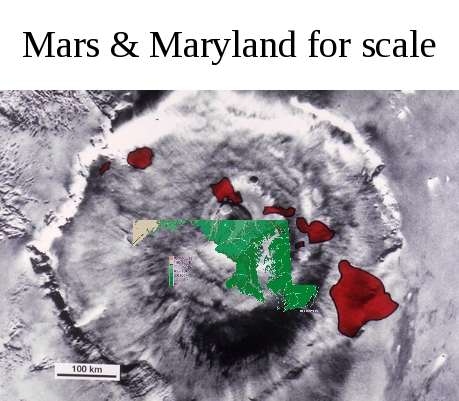
To the right: Olympus Mons with Hawaii and Maryland overlain for scale.
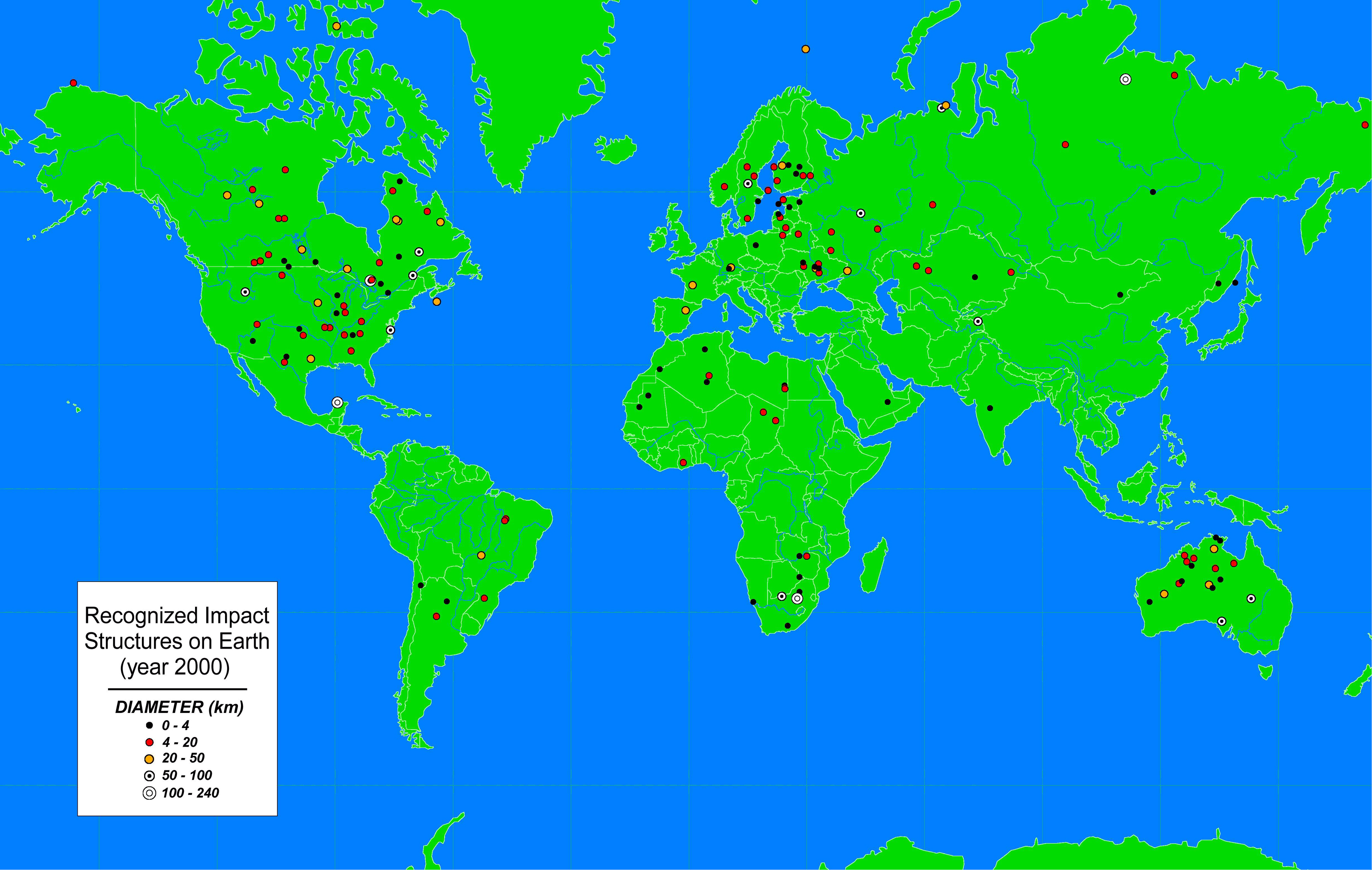
Map of known impact sites on the Earth (click on it for a large resolution). The asymmetry has more to do with how difficult it is to find old impacts than actual statistics of terrestrial impacts.
Chapter 5
- Here are some slides regarding the greenhouse effect. This is overly simplified, but of pressing concern to everyone. For much more detailed information about global warming "is a myth" myths, please consult the excellent website, Skeptical Science.
- Here is a fun website to play with gas-in-a-box. This may give you a better sense of the connection between individual molecular velocities and temperature (or it may not?)
- Figure 5.4 (original at right)
is, perhaps, the worst figure in the book in terms of
egregious errors. Below, for your comparison, is a revised version by
myself. You can click on my version
for a closer view or to save for your own use.
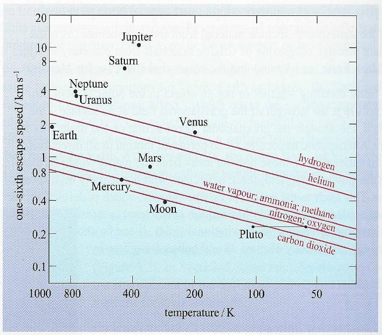
Here's my version of it. You'll be asked to put Titan on this plot in your homework. Click on the image to get a higher resolution for printing, admiring, suitably framing, etc. 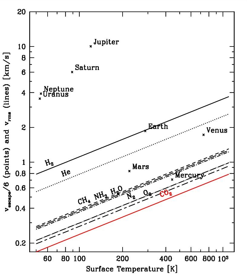
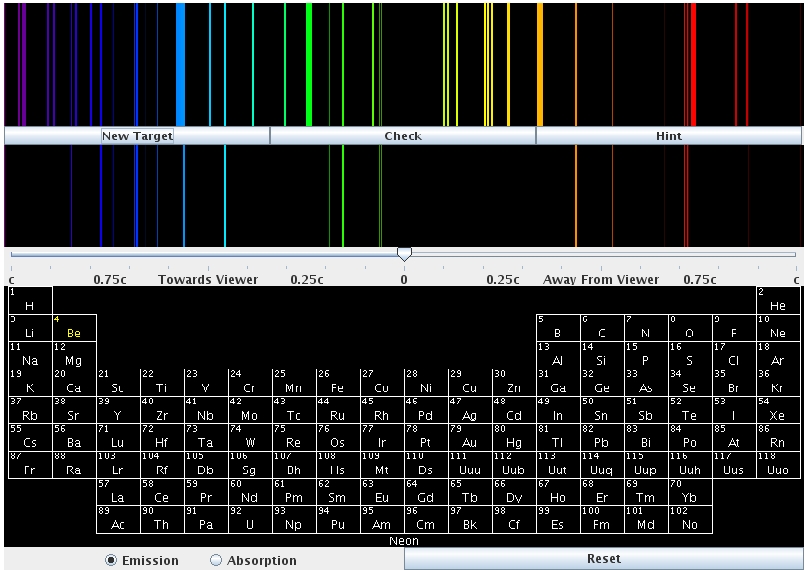
Spectroscopy! Here's a "game" to look at emission (or absorption) lines.
Click here for an animation showing ocean currents over a 2.5 year cycle. It's remarkable how little they shift over that timeframe. While we're not doing currents in class, per se, they are influenced somewhat by the Hadley cells we do talk about. 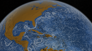
Chapter 6
- Some potentially useful slides will be posted here later.
Here is an awesome (I mean this non-flippantly!) video of the ionosphere as seen by the ISS showing the green oxygen glow and aurorae. Note the glow isn't visible from the ground because you're looking through the atmosphere in the "thin" direction, but the ISS is able to look through hundreds/thousands of miles edge-on. To see it in full screen, click here Chapter 7
- On the far right, stolen brazenly from Mrs. Armes Chemistry and Physics (a NY high school class): an animation demonstrating Kepler's 2nd law.
- On the right below, a plot showing how eccentric an ellipse needs to be before you notice. The colored dots at each (progressively more eccentric) focus reflect eccentricities on the table below. Note that the colors of the corresponding ellipses matches. Note also that the focal points are simply e away from the center since a = 1 here. All the planets orbital eccentricities lie between e= 0 and 0.1 except Mercury (0.2). Note that the only way you can even tell that 0.2 looks like an ellipse is that the Sun (dot) is offcenter!
eccentricity, e color 0.0 red 0.1 green 0.2 blue 0.3 cyan 0.4 pink 0.5 yellow 0.6 red 0.7 green 0.8 blue 0.9 cyan 0.99 pink 0.999 yellow 
The very, very cool libration movie of the Moon's orbit. Note that there is up and down libration as well as side to side. That libration is due to the Moon's orbital tilt. There is also (not in this movie) a libration from moonrise to moonset. These are geometrical librations that do not add to the tidal effect on the Moon. However, the main side to side one does! 
Chapter 8
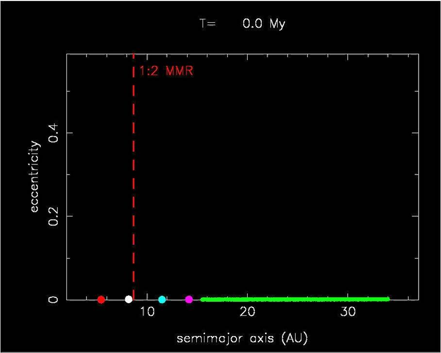
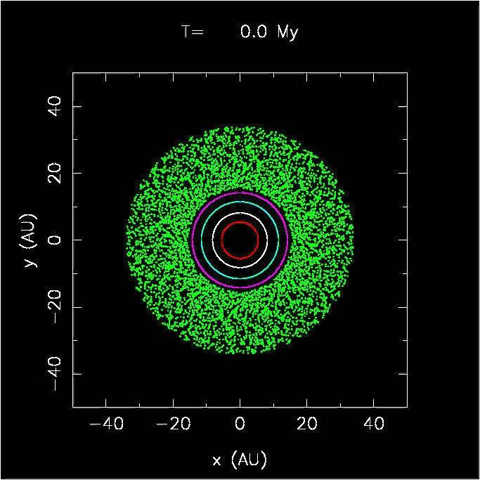
Click on either picture to dowload a quicktime movie of one run of a Nice model. Note the clock at the top of each picture. The movie on the left shows distance of the semi-major axis a vs. eccentricity e; the movie on the right shows a projection from "above" the ecliptic (hence, x vs. y).
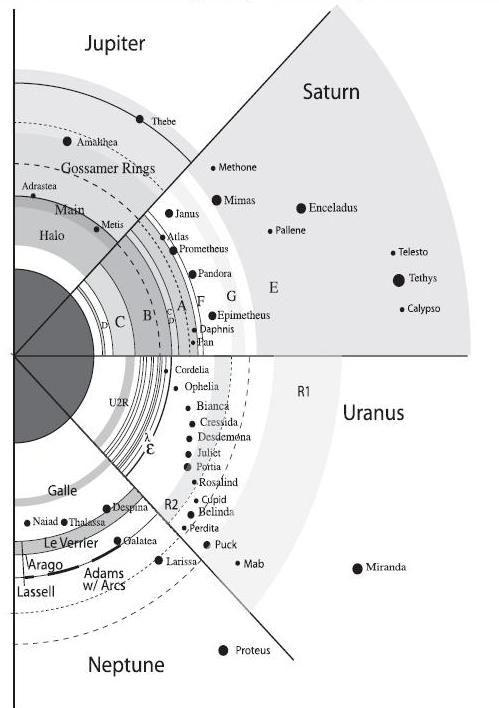
Rings
Here is the supplement on planetary rings.
And here is a recent bit of work on "minijets" in the F ring - a dynamic and interesting puzzle regarding ring stability and longevity.
Here is a breathtaking "film" put together only using real NASA (Cassini and Voyager) images. Note that much of the motion is sped up and ALSO note how pointless it would be to measure the speed of Jupiter's rotation using any belt or zone.
- Some potentially useful slides will be posted here later.
 Back to
main class description webpage
Back to
main class description webpage