ADMIT Design Overview

Introduction

The ALMA Data Mining Toolkit (ADMIT) is a value-added software package which integrates with the ALMA archive and CASA to provide scientists with quick access to traditional science data products such as moment maps, and with new innovative tools for exploring data cubes and their many derived products. The goals of the package are to (1) make the scientific value of ALMA data more immediate to all users, (2) create an analysis infrastructure that allows users to build new tools, (3) provide new types of tools for mining the science in ALMA data, (4) increase the scientific value of the rich data archive that ALMA is creating, and (5) re-execute and explore robustness of the initial pipeline results.

For each ALMA science project a set of science quality image cubes exist. ADMIT runs a series of ADMIT Tasks (AT), which are essentially beefed up CASA tools/tasks, and produces a set of Basic Data Products (BDP). ADMIT provides a wrapper around these tasks for use within the ALMA pipeline and to have a persistent state for re-execution later on by the end user in ADMIT’s own pipeline. ADMIT products are contained in a compressed archive file admit.zip, in parallel with the existing Alma Data Products (ADP). Examples of ADP in a project are the Raw Visibility Data (in ASDM format) and the Science Data Cubes (in FITS format) for each target (source) and each band.

Once users have downloaded the ADMIT files, they can preview the work the ALMA pipeline has created, without the immediate need to download the generally much larger ADP. They will also be able to re-run selected portions of the ADMIT pipeline from either the (casapy) commandline, or a GUI, and compare and improve upon the pipeline-produced results. For this, some of the ADP’s may be needed.

ADMIT Tasks

An ADMIT Task (AT) is made up of zero or more CASA tasks. It takes as input zero or more BDPs and produces one or more output BDPs. These BDPs do not have to be of the same type. An AT also has input parameters that control its detailed functionality. These parameters may map directly to CASA task parameters or may be peculiar to the AT. On disk, ATs are stored as XML. In memory, each is stored in a specific class representation derived from the ADMIT Task base class. A user may have multiple instantiations of any given AT type active in an ADMIT session, avoiding need to to save and recall parameters for different invocations of a task. The Flow Manager keeps track of the connection order of any set of ATs (see Workflow Management). AT parameters are validated only at runtime; there is no validation on export to or import from XML. The representations of every AT are stored in a single XML file (admit.xml).

Basic Data Products

Basic Data Products are instantiated from external files or created as output of an ADMIT Task. As with ATs, the external data format for BDPs is XML and in memory, BDPs are stored in a specific class representation derived from the BDP base class. One XML file contains one and only one BDP. When a BDP is instantiated by parsing of its associated XML file, the file first undergoes validation against a document type definition (DTD). Validation against a DTD will ensure that the XML nodes required to fully instantiate the BDP are present. Since BDP types inherit from a base class (see Figure ref{admitarchitecture}), there is a BDP.dtd which defines the mandatory parameters for all BDPs. For each BDP type, there is also a DTD that defines parameters specific to that BDP type. Individual BDP Types are described in Section ref{s-bdptypes}.

The DTDs for each BDP type will have been autogenerated directly from the class definition Python. Furthermore, the DTD is included in the XML file itself so that the BDP definition is completely self-contained. The ensures integrity against future changes to a BDP definition (i.e., versioning). To allow for flexibility by end users (aka “tinkering”), extraneous nodes not captured in the DTD will be ignored, but will not cause invalidation. Validation against the DTD happens for free with use of standard XML I/O Python libraries. Data validation occurs on both write and read.

BDPs are instantiated by the ATs responsible for creating them. Users will rarely have need to do so themselves. In an AT class, a BDP instantiation from XML may look like:

import parser
b = parser.Parser("myfile.xml")

Parser is a class that uses the SAX library to interpret the XML contents. Inside the XML is a BDPType node that indicates the BDP derived type stored in the XML file, which will be returned by the call. This is essentially the factory design pattern. The XML parser converts a member datum to its appropriate type, then assigns the datum to a variable of the same name in the class. For example:

<noise type="Float">3.255</noise>

is converted to:

BDP.noise = 3.255

In serializing the BDP, we use Python introspection to determine the variable names and data types and write them out to XML, essentially reversing the process. Individual BDP Types are described in Individual BDP Designs

Workflow Management

We take an task-centric view of workflow in which an ADMIT Task (AT) is an arbitrary M-to-N mapping of BDPs, possibly with additional internal attributes and methods. BDPs are passive data containers, without parents or children, and are owned by the AT which produces them. Hence, ATs also function as BDP containers. The Flow Manager (FM) maintains a full list of ATs and how they are connected, allowing it to keep all BDPs up to date as ATs are modified.

Conceptually, a connection maps the output(s) of one AT to the input(s) of another AT. The Flow Manager creates an overall connection map, where a single connection is specified by a six-element element tuple of integers indices:

\((project_{out},AT_{out},BDP_{out},project_{in},AT_{in},BDP_{in})\)

In most cases, the input project and output project will be the same, but in the case of multiflows they can differ. Figure 1 illustrates the connection map concept, while Figures 2 and 3 give an realistic example workflow and the resulting connection map.

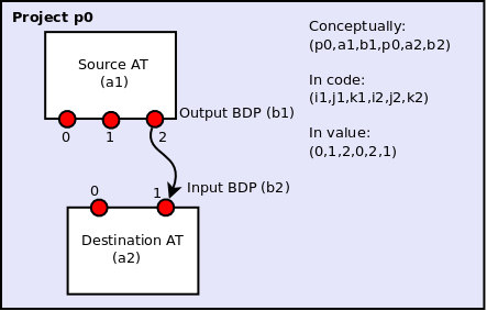
Figure 1: The connection in this diagram connects two ATs, a1 and a2, inside a single project p0. The output BDP of a1 is an input BDP of a2, i.e., \(b1 \equiv b2\). A given output BDP may be the input to an arbitrary number of ATs, but can be the output one and only one AT. For virtual projects, the first and fourth indices in the tuple, i1 and i2, would differ.

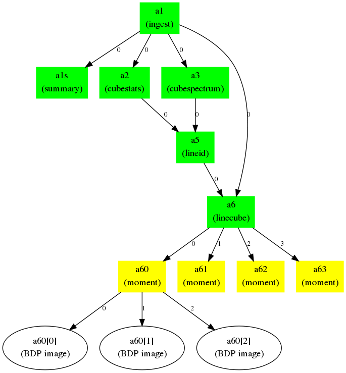
Figure 2: Example realistic workflow with task connection map. A FITS cube is ingested (a1) and processed through a number of tasks: summary, statistics, spectral line cut out, moment. Integers along the arrows indicate the output BDP index available to the next task in the map.

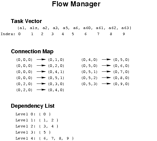
Figure 3: The Flow Manager connection map and dependencies for the workflow in Figure 2. The tuples in the connection map give the project, ADMIT task, and BDP output/input indices. The Flow Manager also computes the dependence list of ATs so that a change in one AT will trigger re-execution of ATs that depend on it in order to recompute the BDPs.

Architecture Overview

Figure 4 is a schematic of the overall interaction of ADMIT modules. Their functionality is described below.

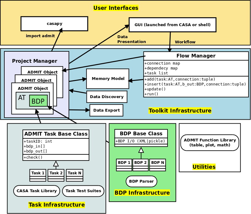
Figure 4: Schematic of how ADMIT fits together.

BDP Infrastructure

The BDP Base Class contains methods and member variables common to all BDPS. Individual BDPs derive from it and add their own special features. BDP I/O is built-in to the base class through Python XML libraries.

Task Infrastructure

ADMIT Task Classes

An ADMIT Task Base Class allows one or more CASA tasks to be encapsulated within one ADMIT Task. The base class should indicate required methods and member variables such that a user can write her own AT. Individual ADMIT Tasks derive from the ADMIT Task Base Class.

Task Test Suites

Each Task must have at least a unit test and integration test.

CASA Task library

From which ADMIT tasks may be built.

Utilities

This ADMIT Function Library includes useful generic classes to handle tables, plotting, and mathematical functions. Utilities will expand as needed.

Toolkit Infrastructure

Data Discovery/Export/Import

This is the module that examines the working directory recursively for FITS files and ADMIT products. It should be able to recognize vanilla, ALMA-style, and VLA-style directory trees and branch accordingly. It will also handle the case of giving a self-contained subset of ADMIT products to a collaborator. It would write a single compressed file containing the ADMIT products in the appropriate hierarchy.

ADMIT Object

From the results of data discovery, the an ADMIT object is instantiated in memory as well as setting up the initial workflow for an ADMIT run (or re-run). This initialization includes instantiation of any discovered ATs and BDPs. One ALMA project maps to one ADMIT object.

Memory Model

How the ADMIT object and state are kept up to date. This is a combination of the Admit Object(s) and the Flow Manager state. The memory model has a one-to-one mapping to what’s on disk.

Flow Manager

This is the infrastructure that strings Tasks together, manages the connection map, decides if an AT and/or its BDPs are out of date and the AT needs to be re-run, and manages task branches.

Project Manager

The PM is a container for one or more ADMIT objects, also referred to as a multiflow. The PM allows for data mining across different ALMA projects.

User Interfaces

casapy

For scripting or direct AT invocation, CASA will be the supported environment. ADMIT specific commands enabled by import admit. There is also the \#!/usr/bin/env casarun environment.

Graphical User Interface.

The GUI consists of two independent parts: 1) The BDP viewer which gives a data summary and 2) the Workflow viewer which shows the connections and state of ATs in the FlowManager, and allows simple modification of ATs in the flow. These are described in detail in sections BDP Viewer Design and Workflow Viewer Design.

Base Classes

AT Base Class

BDP Base Class

Table Base Class

Description

The Table class is a container for holding data in tabluar format. The table can hold data in column-row format and also in plane-column-row format. Data can be added in instantiation, by columns, by rows, or by entire planes.

Use Case

This class is used to store any tabular type data. It should not be used directly but through the Table_BDP class.

Image Base Class

Description

Use Case

Line Base Class

Description

Use Case

Individual AT Designs

File_AT

Description

File_AT creates a File_BDP that contains a reference to an arbitrary file. It has no real use (yet), except for bootstrapping a Flow AT series, where it can be used to test the (large scale) system performance. See also Ingest_AT for a real task that bootstraps a flow.

Use Case

Currently only used by Flow ATs for testing purposes, and thus useful to bootstap a flow, since it can start from an empty directory, and create a zero length file. This means you can create realistic flows, in the same sense as full science flows, and measure the overhead of ADMIT and the FlowManager.

Input BDPs

There are no input BDPs for this bootstrap AT. A filename is required to create an output BDP, using an input keyword (see below).

Input Keywords

• file - The filename of the object. File does not have to exist yet. There is no default.
• touch - Update timestamp (or create zero length file if file did not exist yet)? Default: False.

Output BDPs

• File_BDP - containing the string pointing to the file, following the same convention the other file containers (Image_BDP, Table_BDP) do, except their overhead. There is no formal requirement this should be a relative or absolute address. A symlink is allowed where the OS allows this, a zero length file is also allowed.

Procedure

Simple Unix tools, such as touch, are used. No file existence test done. There are no CASA dependencies, and thus no CASA tasks used.

CASA tasks used

none

Flow_AT

Description

There are a few simple FlowXY_AT’s implemented for experimenting with creating a flow, without the need for CASA and optionally actual files.

This Flow series, together with File_AT, perform nothing more than converting a dummy (one or more) input BDP(s) into (one or more) output BDP(s). Optionally the file(s) associated with these BDP’s can be created as zero length files. Currently three*Flow* ATs are implemented. A simple Flow11_AT can be used for converting a single File_BDP. Two variadic versions are available: Flow1N_AT with 1 input and N outputs, and FlowN1_AT with N inputs and 1 output.

• Flow11_AT - one in, one out
• Flow1N_AT - one in, maNy out
• FlowN1_AT - maNy in, one out
• FlowMN_AT - Many in, maNy out

Use Case

Useful to benchmark the basic ADMIT infrastucture cost of a (complex) flow.

Input BDPs

• File_BDP - containing simply the string pointing to a file. This file does not have to exist. FlowN1_AT can handle multiple input BDPs.

Input Keywords

Depending on which of the FlowXY_AT you have, the following keywords are present:

• file - The filename of the output object if there is only one output BDP (Flow11_AT and FlowN1_AT). For Flow1N_AT the filename is inherited by adding an index 1..N to the input filename, so this keyword will be absent in this Flow1N_AT.
• n - Normally variadic input or output can be determined otherwise (e.g. it generally depends in a complex way on user parameters), but for the Flow series it has to be manually set. Only allowed for Flow1N_AT where the file keyword is not use. Default: 2.
• touch - Update timestamp (or create zero length file if filename did not exist)? Default: False.
• exist - Check existence of the input BDP file(s). Default: True

Output BDPs

• File_BDP - containing simply the string pointing to the file, following the same convention the other file containers (Image_BDP, Table_BDP) do, except their overhead. There is no formal requirement this should be a relative or absolute address. A symlink is allowed where the OS allows this, a zero length file is also allowed.

Procedure

Only Unix tools, such as touch, are used. There are no CASA dependencies, and thus no CASA tasks used.

CASA tasks used

None

Ingest_AT

Description

Ingest_AT converts a FITS file into a CASA Image. It is possible to instead keep this a symlink to the FITS file, as some CASA tasks are able to deal with FITS files directly, potentially cutting down on the I/O overhead. During the conversion to a CASA Image a few extra processing steps are possible, e.g. primary beam correction and taking a subcube instead of the full cube. Some of these steps may add I/O overhead.

Use Case

Normally this is the first step that any ADMIT needs to do to set up a flow for a project, and this is done by ingesting a FITS file into a CASA Image. The SpwCube_BDP contains merely the filename of this CASA Image.

Input BDPs

None. This is an exceptional case (for bootstrapping) where a (FITS) filename is turned into a BDP.

Input Keywords

• file - The filename of the FITS file. No default, this is the only required keyword. Normally with extension .fits, we will refer to this as basename.fits. We leave the issue of absolute/relative/symlinked names up to the caller. We will allow this to be a casa image as well.

• pbcorr - Apply a primary beam correction to the input FITS file? If true, in CASA convention, a basename.flux.fits needs to be present. Normally, single pointings from ALMA are not primary beam corrected, but mosaiced pointings are and thus would need such a correction to make a noise flat image. We should probably allow a way to set another filename

• region - Select a subcube for conversion, using the CASA region notation. By default the whole cube is converted. See also edge= below.

• box - Instead of the more complex region selection described above, a much simpler blc,trc type description is more effective.

  Discussion about region= vs. box=, and is edge= still needed?

• edge - Edge channel rejections. Two numbers can be given, removing the first and last selected number of channel. Default: 0,0 This keyword could interfere with **region=*, but is likely the most common one used*

• mask - If True a mask also needs to be created. need some discussion on the background of this curious option importfits also has a somewhat related zeroblanks= keyword

• symlink - True/False: if True, a symlink is kept to the fitsfile, instead of conversion to a CASA Image. This may be used in those rare cases where your whole flow can work with the fits file, without need to convert to a CASA Image Setting to True, also disables all other processing (mask/region/pbcorr). This keyword should be used with caution, because existing flows will then break if another task is added that cannot use a FITS file. [False]

  theoretically File_AT can also be used to create a File_BDP with a symlinked FITS file, but will subsequent AT’s recognize this underloaded BDP?

• type - If you ingest an alien object of which the origin is not clear, there must be a way to set the type of image (line, continuum, moment, alpha, ...)

Output BDPs

• SpwCube_BDP - the spectral window cube. The default filename for this CASA Image is cim. There are no associated graphical cues for this BDP. Subsequent steps, such as CubeSpectrum_AT and CubeStats_AT. In the case that the input file was already a CASA image, and no subselection or PB correction was done, this can be a symlink to the input filename.

Procedure

Ignoring the symlink option (which has limited use in a full flow), CASA’s importfits will first need to create a full copy of the FITS file into a CASA Image, since there are no options to process a subregion. In the case of multiple CASA programs processing (e.g. when region selection plus primary beam correction), it may be useful to check the performance difference between using tools and tasks.

Although using edge= can be a useful operation to cut down the filesize a little bit, the catch-22 here is that - unless the user knows - the bad channels are not known yet until CubeStats_AT has been run, which is the next step after Ingest_AT. Potentially one can re-run Ingest_AT.

CAVEAT: Using fits files, instead of CASA images, actually adds system overhead each time an image has to be read. The saved time from skipping importfits is quickly lost when your flow contains a number of CASA tasks.

CASA tasks used

• importfits - if just a conversion is done. No region selection can be done here, only some masking operation to replace masked values with 0s.
• imsubimage - only if region processing is done. Note box= and region= and chans= have common methods, our Ingest_AT should keep that simpler. For example, chans=”11~89” for a 100 channel cube would be same as edge=11,10
• immath - if a primary beam correction is needed, to get noise flat images.

Alternatively, AT’s can also use the CASA tools. Especially this can be a more efficient way to chain a number of small image operations, as for example Ingest_AT would do if region selection and primary beam correction are used.

CubeSpectrum_AT

Description

CubeSpectrum_AT will compute one (or more) typical spectra from a spectral line cube. They are stored in a CubeSpectrum_BDP, which also contains a graph of intensity versus frequency. For certain types of cubes, these can be effectively used in LineID_AT to identify spectral lines.

The selection of which point will be used for the spectrum is of course subject to user input, but some automated options can be given. For example, the brightest point in the cube can be used. The reference pixel can be used. The size around this point can also be choosen, but this is not a recommended procedure, as it can affect the LineID_AT procedure, since it will smooth out (but increase S/N) the spectrum if large velocity gradients are present. If more S/N is needed, CubeStats_AT or PVCorr_AT can be used.

Note in an earlier version, the SpectralMap_AT would allow multiple points to be used. We deprecated this, in favor of allowing this AT to create multiple points instead of just one. Having multiple spectra, much like what is done in PVCorr_AT, cross-correlations could be made to increase the line detection success rate.

This AT used to be called PeakSpectrum in an earlier revision.

Use Case

This task is probably one of the first to run after ingestion, and will quickly be able to produce a representative spectrum through the cube, giving the user ideas how to process these data. If spectra are taken through multiple points, a diagram can be combined with a CubeSum centered around a few spectra.

Input BDPs

• SpwCube_BDP - The cube through from which the spectra are drawn. Required. Special values xpeak,ypeak are taken from this cube.
• CubeSum_BDP - An optional BDP describing the image that represents the sum of all emission. The peak(s) in this map can be selected for the spectra drawn. This can also be a moment-0 map from a LineCube.
• FeatureList_BDP - An optional BDP describing features in an image or cube, from which the RA,DEC positions can be used to draw the spectra.

Input Keywords

• points - One (or more) points where the spectrum is computed. Special names are for special points: xpeak,ypeak are for using the position where the peak in the cube occurs. xref,yref are the reference position (CRPIX in FITS parlor).
• size - Size of region to sample over. Pixels/Arcsec. Square/Round. By default a single pixel is used. No CASA regions allowed here, keep it simple for now.
• smooth - Some smoothing option applied to the spectrum. Use with caution if you want to use this BDP for LineID.

Output BDPs

• CubeSpectrum_BDP - A table containing one or more spectra. For a single spectrum the intensity vs. frequency is graphically saved. For multiple spectra (the original intent of the deprecated SpectralMap_AT) it should combine the representation of a CubeSum_BDP with those of the Spectra around it, with lines drawn to the points where the spectra were taken.

Procedure

After making a selection through which point the spectrum is taken, grabbing the values is straightforward. For example, the imval task in CASA will do this.

CASA tasks used

• imval - to extract a spectrum around a given position

CubeStats_AT

Description

CubeStats_AT will compute per-channel statistics, and can help visualize what spectral lines there are in a cube. They are stored in a CubeStats_BDP. For certain types of cubes, these can be effectively used in LineID_AT to identify spectral lines. In addition, tasks such as CubeSum_AT and LineCube_AT can use this if the noise depends on the channel.

Use Case

Many programs needs to know (channel dependent) statistics from a cube in order to be able to clip out the noise and get as much signal in the processing pipeline. In addition, the analysis to compute channel based statistics needs to include some robustness, to remove signal. This will become progressively hard if there is a lot of signal in the cube.

Input BDPs

• SpwCube_BDP - input spectral window cube, for example as created with Ingest_AT.

Input Keywords

• robustness - Several options can be given here, to select the robust RMS. (negative half gauss fit, robust, ...)

Output BDPs

• CubeStats_BDP - A table containing various quantities (min,max,median,rms) on a per channel basis. A global statistics can (optionally?) also be recorded. The graphical output contains at least two plots:

1. histogram of the distribution of Peak (P), Noise (N), and P/N, typically logarithmically;
2. A line diagram shows the P, N and P/N (again logarithmically) as function of frequency. As a good diagnostic, the P/N should now not depend on frequency if only line-free channels are compared. It can also be a good input BDP to LineID_AT.

Procedure

The imstat task (or the ia.statistics tool) in CASA can compute plane based statistics. Although the medabsdevmed output key is much better than just looking at \(\sigma\), a signal clipping robust option may soon be available to select a more robust way to compute what we call the Noise column in our BDP. Line detection (if this BDP is used) is all based on log(P/N).

CASA tasks used

• imstat - extract the statistics per channel, and per cube. Note that the tool and task have different capabilities, for us, we need to the tool (ia.statistics) Various new robustness algorithms are now implemented using the new algorithm= keyword.

CubeSum_AT

Description

CubeSum_AT tries to create a representative moment-0 map of a whole cube, by adding up all the emission, irrespective

Use Case

A simple moment-0 map early in a flow can be used to select a good location for selecting a slice through the spectral window cube. See PVSlice_AT.

Input BDPs

• SpwCube - input cube
• CubeStats - Peak/RMS. Optional. Useful to be more liberal and allow cutoff to depend on the RMS, which may be channel dependent.

Input keywords

• cutoff - Above which emission (or below which, in case of absorbtion features).
• absorption - Identify absorption lines? True/False

Output BDPs

• CubeSum_BDP - An image

Procedure

The method is a special case of Moment_AT, but we decided to keep it separate. Also when the noise level accross the band varies, the use of a CubeStats_BDP is essential. Althiough it is optional here, it is highly recommended.

CASA Tasks Used

FeatureList_AT

Description

FeatureList_AT takes a LineCube, and describes the three-dimensional structure of the emission (and/or absorption)

Note

Should we allow 2D maps as well?

Use Case

Input BDPs

Depending on which BDP(s) is/are given, and a choice of keywords, line identification can take place. For example, one can use both a CubeSpectrum and CubeStats and use a conservative AND or a more liberal OR where either both or any have detected a line.

• CubeSpectrum - A spectrum through a selected point. For some cubes this is perfectly ok.
• CubeStats - Peak/RMS. Since this table analyzed each plane of a cube, it will more likely pick up weaker lines, which a CubeSpectrum will miss.
• PVCorr - an autocorrelation table from a PVSlice_AT. This has the potential of detecting even weaker lines, but its creation via PVSlice_AT is a fine tuneable process.

Note

• SpectralMap - This BDP may actually be absorbed in CubeSpectrum, where there is more than one spectrum, where every spectrum is tied to a location and size over which the spectrum is computed.

Input keywords

• vlsr - If VLSR is not know, it can be specified here. Currently must be known, either via this keyword, or via ADMIT (header).

Note

Is that in admit.xml? And what about VLSR vs. z?

• pmin - Minimum likelihood needed for line detection. This is a number between 0 and 1. [0.90]
• minchan - Minimum number of continguous channels that need to contain a signal, to combine into a line. Note this means that each channel much exceed pmin. [5]

Output BDPs

• LineList_BDP - A single LineList is produced, which is typically used by LineCube_AT to cut a large spectral window cube into smaller LineCubes.

Procedure

The line list database will be the splatalogue subset that is already included with the CASA distribution. This one can be used offline, e.g. via the slsearch() call in CASA. Currently astropy’s astroquery.splatalogue module has a query_lines() function to query the full online web interface.

Once LineID_AT is enabled to attempt actual line identifications, one of those methods will be selected, together with possible selections based on the astrophysical source. This will likely need a few more keywords.

A few words about likelihoods. Each procedure that creates a table is either supposed to deliver a probability, or LineID_AT must be able to compute it. Let’s say for a computed RMS noise \(\sigma\), a \(3\sigma\) peak in a particular channel would have a likelihood of 0.991 (or whatever value) for CubeStats.

CASA Tasks Used

There are currently no tasks in CASA that can handle this.

LineID_AT

Description

LineID_AT creates a LineList_BDP, a table of spectral lines discovered or detected in a spectral window cube. It does not need a spectral window cube for this, instead it uses derived products (currently all tables) such a CubeSpectrum_BDP, CubeStats_BDP or PVCorr_BDP. It is possible to have the program determine the VLSR if this is not known or specified (in the current version it needs to be known), but this procedure is not well determined if only a few lines are present. Note that other spectral windows may then be needed to add more lines to make this fit un-ambigious.

Cubes normally are referenced by frequency, but if already by velocity then the rest frequency and vlsr/z must be given.

For milestone 2 we will use the slsearch() CASA task, a more complete database tool is under development in CASA and will be implemented here when complete.

Use Case

In most cases the user will want to identify any spectral lines found in their data cube. This task will determine what is/is not a line and attempt to identify it from a catalog.

Input BDPs

• CubeSpectrum_BDP - just a spectrum through a selected point.
• CubeStats_BDP Peak/RMS. Since this table analyses each plane of a cube, it will more likely pick up weaker lines, which a CubeSpectrum_BDP will miss.
• PVCorr_BDP an autocorrelation table from a PVSlice_AT. This has the potential of detecting even weaker lines, but its creation via PVSlice_AT is a fine tuneable process.

Input Keywords

• vlsr - If VLSR is not known, it can be specified here. Currently must be known, either via this keyword, or via ADMIT (header). This could also be z, but this could be problematic for nearby sources, or for sources moving toward us.
• rfeq - Rest frequency of the vlsr, units should be specified in CASA format (95.0GHz) [None]. Only required if the cube is specified in velocity rather than frequency.
• pmin - Minimum sigma level needed for detection [3], based on calculated rms noise
• minchan - Minimum number of contiguous channels that need to contain a signal, to combine into a line. Note this means that each channel must exceed pmin. [5]

Output BDP

LineList_BDP - A single LineList is produced, which is typically used by LineCube_AT to cut a large spectral window cube into smaller LineCube’s.

Output Graphics

None.

Proceedure

Depending on which BDP(s) is/are given, and a choice of keywords, the procedure may vary slightly. For example, one can use both a CubeSpectrum_BDP and CubeStats_BDP and use a conservative AND or a more liberal OR where either both or any have “detected” a line. The method employed to detect a line will be based on the line finding mechanisms found in the pipeline. The method will be robust for spectra with sparse lines, but may not be for spectra that are a forest of lines. Once lines are found the properties of each line will be determined ( rest frequency, width, peak intensity, etc.). Using the parameters (rest frequency and width) the database will be searched to find any possible line identifications.

CASA Tasks Used

• slsearch to attempt to identify the spectral line(s)

LineCube_AT

Description

A LineCube is a small spectral cube cut from the full spectral window cube, typically centered in frequency/velocity on a given spectral line. LineCube_AT creates one (or more) of such cubes. It is done after line identification (using a LineList_BDP), so the appropriate channel ranges are known. Optionally this AT can be used without the line identification, and just channel ranges are given (and thus the line will be designated as something like “U-115.27”. The line cubes are normally re-gridded onto a common velocity (km/s) scale, for later comparison, and thus the CubeStats_AT will need to be re-run on these cubes. Also, normally the continuum will have been subtracted these should only be the line emission, possibly with contamination from other nearby lines. This is a big issue if there is a forest of lines, and proper separation of such lines is a topic for the future and may be documented here as well with a method.

One of the goals of LineCube_AT is to creates identically sized cubes of different molecular transitions for easy comparison and cross referenced analysis.

Use Case

A LineCube would be used to isolate a single molecular component in frequency dimensions. The produced subimage would be one of the natural inputs for the Moment_AT task.

Input BDPs

• SpwCube_BDP - a (continuum subtracted) spectral window cube
• LineList_BDP - a LineList, as created with LineID_AT. This LineList does not need to have identified lines. In the simple version of LineID will just designate channel ranges as “U” lines.
• CubeStats_BDP - (optional) CubeStats associated with the input spectral cube. This is useful if the RMS noise would depend on the channel, which can happen for wider cubes, especially near the spectral window edges. Otherwise the keyword cutoff will suffice.

Input Keywords

• regrid (optional) - The velocity to regrid the output cube channels to, units: can be specified as other CASA values are (3.0kms), but defaults to km/s [None] (i.e. no regridding)
• cutoff (optional) - The cutoff value in sigma to use when generating the subcube(s), all values below this will be masked [5.0]

Output BDP

LineCube_BDP - The output from this AT will be a line cube for each input spectral line. Each spectral cube will be centered on the spectral line and regridded to a common velocity scale, if requested.

Output Graphics

None

Procedure

For each line found in the input LineList_BDP this AT will grab a subcube based on the input parameters.

CASA Tasks Used

• imsubimage - to extract the final subcube from the main cube, including any masking
• imregrid - if regridding in velocity is needed

PVSlice_AT

Description

PVSlice_AT creates a position-velocity slice through a spectral window cube, which should be a representative version showing all the spectral lines.

Use Case

A position-velocity slice is a great way to visualize all the emission in a spectral window cube, next to CubeSum.

Input BDPs

• SpwCube_BDP - Spectral Window Cube to take the slice through. We normally mean this to be a Position-Position-Velocity (or Frequency) cube.
• CubeSum - Optional. One of CubeSum or PeakPointPlot can be used to estimate the best slit. It will use a moment of inertia analysis to decipher the best line in RA-DEC for the slice.
• PeakPointPlot - Optional

Input Keywords

• center - Center and Position angle of the line in RA/DEC. E.g. 129,129,30 Optional length? Else full slice through cube is taken * NEED TO DESCRIBE HOW POSITION ANGLE IS DEFINED. EAST OF NORTH?*
• line - Begin and End points of the line in RA/DEC. E.g. 30,30,140,140\ WHAT ARE THE UNITS? COULD THIS BE DONE WITH A REGION KEYWORD?
• major - Place the slit along the major axis? Optionally the minor axis slit can be taken. For rotation flow the major axis makes more sense, for outflows the minor axis makes more sense. Default: True.
• width - Width of the slit. By default sampling through the cube is done, which equals a zero thickness, but a finite number of pixels can be choosen as well, in which case the signal within that width is averaged. Default: 0.0
• minval - Minimum intensity value below which no data from CubeSum or PeakPointPlot are used to determine the best slit.
• gamma - The factor by which intensities are weighed (intensity**gamma) to compute the moments of inertia from which the slit line is computed. Default: 1

Output BDP

• PVSlice_BDP -

Procedure

Either a specific line is given manually, or it can be derived from a reference map (or table). By this it computes a (intensity weighted) moment of inertia, which then defines a major and minor axis. Spatial sampling on output is the same as on input (this means if there ever is a map with unequal sampling in RA and DEC, there is an issue, WSRT data?).

CASA Tasks Used

• impv - to extract the PV slice

PVCorr_AT

Description

PVCorr_AT uses a position-velocity slice to correlate distinct repeating structures in this slice along the velocity (frequency) direction to find emission or absorbtion lines.

Caveat: if the object of interest has very different types of emission regions, e.g a nuclear and disk component which do not overlap, the detection may not work as well.

Use Case

For weak lines (NGC253 has nice examples of this) none of the CubeStats or CubeSpectrum give a reliable way to detect such lines, because they are essentially 1-dimensional cuts through the cube and become essentially like noise. When looking at a Position-Velocity slice, weak lines show up quite clearly to the eye, because they are coherent 2D structures which mimick those of more obvious and stronger lines in the same PVSlice. The idea is to cross-correlated an area around such strong lines along the frequency axis and compute a cross-correlation coefficient.

There is also an interesting use case for virtual projects: imagine a PV slice with only a weak line, but in another related ADMIT object (i.e. a PVslice from another spectrum window) it is clearly detected. Formally a cross correlation can only be done in velocity space when the VLSR is known, but within a spectral window the non-linear effects are small. Borrowing a template from another spw with widely different frequencies should be used with caution.

Input BDPs

• PVSlice - The input PVSlice
• PVslice2 - Alternative PVSlice (presumably from another virtual project)
• CubeStats - Statistics on the parent cube

Input Keywords

• cutoff - a conservative cutoff above which an area is defined for the N-th strongest line. Can also be given in terms of sigma in the parent cube.
• order - Pick the N-th strongest line in this PV slice as the template. Default:1

Output BDPs

• PVCorr_BDP - Table with cross-correlation coefficients

Procedure

After a template line is identified (usually the strongest line in the PV Slice), a conservative polygon (not too low a cutoff) is defined around this, and cross correlated along the frequency axis. Currently this needs to be a single polygon (really?)

Given the odd shape of the emission in a PVSlice, the correlation coefficient is not exactly at the correct velocity. A correction factor needs to be determined based on identifying the template line with a known line frequency, and VLSR. Since line identifaction is the next step after this, this catch-22 situation needs to be resolved, otherwise a small systemic offset can be present.

CASA tasks used

none exist yet that can do this. NEMO has a program written in C, and the ideas in there will need to be ported to python.

PeakPointPlot_AT

Moment_AT

Individual BDP Designs

Table_BDP

Image_BDP

Line_BDP

LineList_BDP

Description

A table of spectral lines detected in a spectrum, map, or cube. Output from the LineID_AT.

Inherits From

Table_BDP

Constituents

The items of this BDP will be a table with the following columns:

• frequency - in GHz, precise to 5 significant figures
• uid - ANAME-FFF.FFF ; e.g. CO-115.271, N2HP-93.173, U-98.76
• formula - CO, CO_v1, C2H, H13CO+
• fullname - Carbon monoxide, formaldehyde
• transition - Quantum numbers
• velocity - vlsr or offset velocity (based on rest frequency)
• energies - lower and upper state energies in K
• linestrength - spectral line strength in D$^2$
• peakintensity - the peak intensity of the line in Jy/bm
• peakoffset - the offset of the peak from the rest frequency in MHz
• fwhm - the FWHM of the line in km/s
• channels - the channels the line spans (typically FWHM)

Additionally an item to denote whether the velocity is vlsr or offset velocity. The offset velocity will only be used when the vlsr is not known and cannot be determined. The coordinates of where the line list applies along with units will also be stored.

LineCube_BDP

Description

A Line Cube is a subcube of the initial image, This subcube represents the emission of a single (or degenerate set) spectral line, both in spatial and velocity/frequency dimensions. It is the output from the LineCube_AT.

Inherits From

SpwCube_BDP

Constituents

An image of the output cube, a SPW cube, a listing of the molecule, transition, energies, rest freq, and line width.

SpwCube_BDP

CubeSpectrum_BDP

CubeStats_BDP

PVCorr_BDP

Graphical User Interface Design

BDP Viewer Design

The purpose of the BDP viewer is to give the user an always up-to-date summary of the data that have been produced by ADMIT for the target ingested file(s). In this model, each view window is associated with one ADMIT object. As the user produces data by creating and executing ATs through a flow, the view representing the data will be refreshed. Tasks which create images or plots will also create thumbnails which can be shown in the view and clicked on to be expanded or to get more information. We adopt a web browser as the basic view platform because

1. Much of the interaction, format (e.g., tabbed views), and bookkeeping required is already provided by a web browser platform, decreasing greatly the amount of code we have to write.
2. Users are quite familiar with browsers, making learning the BDP viewer easier. Furthermore, they can user their browser of choice.
3. By doing so, we can adopt the look and feel of the ALMA pipline web log, keeping to a style with which ALMA users will be familiar.
4. Python provides an easy-to-use built-in HTTP server (BaseHTTPServer), so no external Python package is needed.
5. Writing the data summary in HTML allows us flexibility to test various view styles and quickly modify the style as our needs change.

When an ADMIT object is instantiated, it will start a BDP view server on a unique localhost port in a separate thread and report to the user the localhost web address on which to view the BDPs for that ADMIT object. The server will be given the data output directory as its document root. Upon execution, each AT will invoked a method on the ADMIT object that updates an HTML file(s) in the document root with the newly available items. Users can monitor different ADMIT objects in different browser tabs.

The HTML files will include the well-known Javascript code Live.js which auto-refreshes pages when something has changed. This script polls once per second for changes in local HTML, CSS, or Javascript. If we find resource usage is an issue, we could increase the poll interval. We can also modify the script to monitor other file types, but it is simpler to use a timestamp in a comment tag in index.html that gets modified at at each update.

Following the ALMA Archive Pipeline web pages, we will use the Bootstrap Framework for the layout style. The general layout will be grid-like. Each AT writes its summary information in its own division (“div” in CSS language) in the web page, and divisions are added at the bottom as they are created. So the order of divisions on the web page are essentially workflow order (for simple flows). In each division, the BDP info will be laid out horizontally as thumbnails or links to secondary pages. For multiflows, we may want a customization in which all ADMIT objects in the multiflow are represented on the page with clear graphical separation.

Workflow Viewer Design

Lisa to put FlowManger conceptual design here.

Example Code

This is working example that ingests a FITS file, makes moments, saves the ADMIT state, restores it, modifies the moment parameters and then remakes the moments.

#! /usr/bin/env casarun
#
#    Example script to execute the things we want for Milestone 1 (Oct 31, 2014)
#    Modified to work for the codebase for Milesyton2 (Apr 30, 2015)
#


import admit.Admit as ad
from admit.at.Ingest_AT import Ingest_AT
from admit.at.Moment_AT import Moment_AT
from admit.at.Moment_AT import Moment_AT
from admit.AT import AT                      # @todo normally not needed

                                # 4 ways to be called
a = ad.Admit()                  # Look for "foobar.admit" in which there must be an admit.xml
                                # or look for "foobar.fits" if it's a new project
                                # or leave blank for current directory and existing admit.xml
                                # existing admit.xml in current directory
if a.new:
    print "New ADMIT"
    a.plotmode(0)                             # 1=interactive plots on screen (0=batch mode)
    cutoff = 0.05
    a.set(cutoff=cutoff)

    i0 = a.addtask( Ingest_AT(file='foobar.fits') )
    a.run()                               
    a.set(i0=i0)                              # save for the second run


    i1 = a.addtask( Moment_AT(), [(i0,0)] )      
    a[i1].setkey('moments',[0])
    a[i1].setkey('cutoff',[cutoff])
    #a[i1].setChanRange([9,40])

    i2 = a.addtask( Moment_AT(), [(i0,0)] )
    a[i2].setkey('moments',[1])
    a[i2].setkey('cutoff',[cutoff])
    #a[i2].setChanRange([9,40])

    i3 = a.addtask( Moment_AT(), [(i0,0)] )
    a[i3].setkey('moments',[2])
    a[i3].setkey('cutoff',[cutoff])
    #a[i3].setChanRange([9,40])

    a.run()
    a.write()

    # test08:

    if True:
        # should not do anything
        print "BEGIN test08"
        a.run()
        print "END test08"

    # test09:     

    if True:
        print "BEGIN test09"
        fn = 'cim.mom.0'                   # remove some file, we want to test if the flow recomputes
        os.system('rm -rf %s' % fn)
        a.run()                            # should remake this mom=1 map. 
        print "END test09"

    # test10 : remove a task

    if True:
        a.fm.remove(i2)     
        print "BEGIN test11"
        a.run()                        #  nothing should have run here
        print "END test11"

    # test11: change the input fits file

    if True:
        # @todo:  if foobar2.fits doesn't exist, symlink it from foobar.fits
        a[i0].setkey('file','foobar2.fits')
        a.run()          
        a.write()
else:
    # @todo   the plotmode is not read from admit.xml
    # @todo   doesn't seem to run 3rd time?  claims:    Exception: No BDP inputs set

    # the project existed, so pick up where we left, and do a few other things
    print "Existing ADMIT"
    a.plotmode(0)                             # @todo  this is not done by admit.xml

    # test20: restoring an ADMIT variable

    if True:
        # set a new value
        a.set(foobar=[1,2,3])
        print 'FOOBAR=',a.get('foobar')
        # retrieve the old one from the previous run
        cutoff = a.get('cutoff')
        print "CUTOFF=",cutoff
    a.run()                                         # should do nothing


    # test21: remove a file    @todo rerun this and it will fail

    if True:
        print "BEGIN test21"
        fn = 'cim.mom.0'             # remove some file, we want to test if the flow recomputes
        os.system('rm -rf %s' % fn)
        a.run()                      # should remake this mom=1 map. 
        print "END test21"

    # test20: insert a task

    if True:
        i0 = a.get('i0')                                 # retrieve from previous run (like a GUI click on task)
        i2 = a.addtask(Moment_AT(), [(i0,0)] ) 
        a[i2].setkey('moments',[-1])
        a[i2].setChanRange([9,40])                       # PJT: yuck cheat, uniform key interface pls
        a.run()                                          # this should only run the new mom=-1

    a.write()