Probably the most important thing to remember at various stages of your calibration is careful and consistent data inspection. The end-goal of calibration is to create flat phases and/or flat amplitudes for the calibrators as function function of frequency and/or time. Use uvflag and friends where needed to edit out discrepant data that could throw of calibration routines.
For the calibrator(s), inspect the run of phase and amplitude as a function of time and channel. In this example we are using the ``sma'' flavor of uvplt and uvspec:
 % smauvplt  vis=cx012.SS433.2006sep07.1.miriad select="source(3c273)" axis=time,phase interval=3
 % smauvplt  vis=cx012.SS433.2006sep07.1.miriad select="source(3c273)" axis=time,amp   interval=3

 % smauvspec vis=cx012.SS433.2006sep07.1.miriad select="source(3c273)" axis=chan,phase interval=999
 % smauvspec vis=cx012.SS433.2006sep07.1.miriad select="source(3c273)" axis=chan,amp   interval=999
Recall that ``taskname -k'' will give you a full description of all the program parameters.
To inspect the amplitudes in a totally different manner, construct a 3D cube from the visibility data and view this with any of the FITS or MIRIAD image viewers that are available. Here is an example using ds9:
 % ds9 &
 % uvimage vis=cx012.SS433.2006sep07.1.miriad out=cube1 select="-source(noise),-auto"
 % histo in=cube1
 % mirds9 cube1
Another useful (but busy) program for checking your data quality is the closure phase, which we expect to be zero on average:
% closure vis=cx012.SS433.2006sep07.1.miriad select="source(3c273),-auto" device=/xs
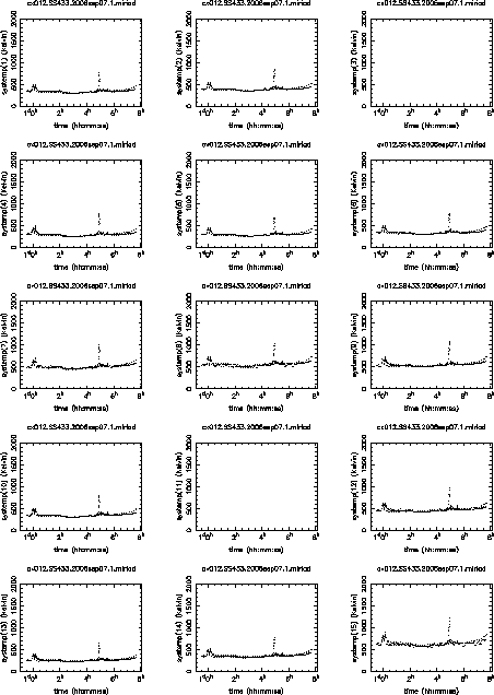
To inspect a wide range of uv variables use varplt (a list can be found in Appendix D):
% varplt vis=cx012.SS433.2006sep07.1.miriad device=/xs yaxis=systemp nxy=5,3 yrange=0,2000 options=compress
shows C3 and C11 are not online. Autoscaling showed C2 has a bad point. But overall something bad happened around 5h UT. See Figure 2.1