
J and Astronomy
J is an extremely terse programming language. It is interactive, i.e., you
type in an expression and it is executed as soon as you hit ``return''.
One strength is that whole arrays of numbers can be represented by a single
name and can be manipulated without any explicit reference to the indices of
individual elements of the array. J is descended from APL, and like it has
a rich array of operations.
Unlike APL, it uses only the normal ASCII character set -- operators are
the usual symbols, plus others formed by appending a period or colon after
ASCII symbols, i.e., + , +. and +: are distinct functions. Thus "B % A" where
B and A are numbers or arrays represents B divided by A, while "%. A" is the
inverse of the matrix A and "B %. A" computes the solution of the linear system
A x = B. As another example, "a ^ b" is a to the power b, but "a ^:n" applies
the operation "a" n times, while "a ^:_" iterates "a" until convergence, reducing
the notational apparatus drastically. J is *free*. It runs under Linux, OS X, and Windows.
Get J at
http://www.jsoftware.com.
AND... You can run J on your iPhone or Android phone.
It's a free download. These apps are the full J language; all the code on this
page (except a few cases where I call a FORTRAN routine) will run on these phones.
(On my ancient iPhone 4S, J could invert a 500 x 500 matrix in 5.5 sec - and that's in
double precision. On my new Pixel 8 Pro, this operation takes about 0.16 sec.)
For the iPhone or iPad, see https://code.jsoftware.com/wiki/Guides/iOS
For an Android phone, see https://code.jsoftware.com/wiki/Guides/JAndroid
Here are some definitions needed for my code on this page -- load this file first:
local_defs.ijs. Also note that where I have
written a file name as "/your_path/..." you should replace this by
the full path name to the folder where you have put the .ijs script in question.
Also, in any J code like that posted here, whatever follows "NB." is just a comment.
Check back later as this page is continuously updated.
What Aulus Gellius (ca 160 CE) wrote about the study of logic
applies nicely to the study of J:
"... and I need only add by way of advice, that the study and knowledge
of this science in its rudiments does indeed, as a rule, seem forbidding
and contemptible, as well as disagreeable and useless. But when you have
made some progress, then finally its advantages will become clear to you,
and a kind of insatiable desire for acquiring it will arise; so much so,
that if you do not set bounds to it, there will be great danger lest, as
many others have done, you should reach a second childhood amid those
mazes and meanders of logic, as if among the rocks of the Sirens."
"Attic Nights" Bk XVI, viii, 15-17.
And then there's Zippy.
Astronomy
Here's a routine to correct coordinates for precession:
precess.ijs.
This is for the integration of the Lane-Emden (polytrope) equation:
polytrope.ijs.
and this is for the case of the isothermal sphere:
iso_sphere.ijs.
This code evaluates scattering and absorption light by spheres using Mie theory:
mie.ijs.
This Mie theory code evaluates scattering of polarized light by spheres as
a function of the scattering angle:
angle_scat.ijs.
This code evaluates the Voigt function, which describes the shape of spectral
lines: voigt.ijs.
(Keplers_Equation.ijs) -
This J code solves Kepler's Equation: KE=: ,~ (p. sin)^:_ ]
(Yes, that is the entire program!)
Here's a routine to evaluate the Chandrasekhar H(µ) function:
H_funct.ijs. (With this function we may evaluate
the intensity of light scattered in any direction from a thick, isotropically
scattering atmosphere illuminated by radiation incident at an arbitrary angle.
For Rayleigh scattering of a beam with polarization see "ARay.ijs" below.)
This code gives the location in the sky of the sun, moon & planets. It also
displays the moon's shape
and orientation:
Sky.ijs. It needs some data files:
SS_DAT.
Here's a version that also plots the location of
the sun, moon and planets against the background of all stars brighter than 5.2
magnitudes: Skys.ijs.
This little routine gives the times at which the Milky Way crosses the observer's
meridian and it's angle (azimuth): Milky_Way.ijs.
Why? A tool for investigating the possible alignments of ancient structures,
e.g., The Great Hopewell Road.
Multi-level atoms
The following code deals with the solution of an n-level atom or ion under
conditions relevant to the interstellar medium.
The J routines are here:
N_pop.ijs.
There must be a file of atomic data
for each ion considered. Some are given in this directory:
ATOMIC_DATA.
Just a note on the sort of output produced:N_pop.txt.
Here is a discussion of the theory
behind these routines: N-level.pdf.
Transfer of radiation in plane-parallel atmospheres
Here are some routines for evaluating the radiation field in plane-parallel
atmospheres, based on the integral equations of the problem. We assume the
source function and/or Planck function can be well approximated by a cubic
spline. A J routine "SpMD.ijs" (see below) is used to
construct matrix representations of the integral of the function against
against a kernel function, based on this spline representation.
For example the routine IQMsi.ijs creates a matrix
which operates on the source function to give the emergent intensity from a
semi-infinite, plane parallel atmosphere, I(mu), as a function of the emergent
angle mu = cos[theta].
Here is another routine, MTsi.ijs, which creates the
matrix representations of the integration of a source function against various
exponential integrals. For example, the $\Phi$ transform evaluates the flux at
each level in the atmosphere by integration of the source function against the
2nd exponential integral. Perhaps the most important transform is the
$\Lambda$-transform, which gives the mean intensity at a given point in the
atmosphere by integration over the source function. For a given grid of optical
depths "tau", the expression "1 MTsi tau" gives $\Lambda$-transform and
"2 MTsi tau" gives the $\Phi$-transform. Other integers on the left of MTsi
give transforms involving higher order exponential integrals useful for applications
involving polarization (see below). Note that MTsi assumes a semi-infinite
atmosphere and thus integrates from the last (largest) tau point to infinity,
using a linear extrapolation of the source function.
Polarization
If the polarization of the scattered radiation is taken into account, the
equations become more complicated. If the scattering is by free electrons
or molecules, the scattering will follow Rayleigh's law. The integral equations
in this case can be found in Harrington (1970) Astrophysics & Space Science, 8,
227-242. (See also
Harrington (1969).)
In addition to the Lambda-transform, we introduce two additional
transforms, the "M-transform" and the "N-transform", which involve higher
exponential integrals. The J code to create the matrix representation is
"3 MTsi tau" for the "M-transform" and "5 MTsi tau" for "N-transform".
In addition, to evaluate the flux of polarized radiation, we also need the
"$\Lambda^{(4)}$-transform" (the integral against the E4 kernel), given by
"4 MTsi tau". The messy details of the equations behind all this are given
in these notes.pdf.
If the run of the Planck function with optical depth, B(tau), and the fractional
scattering, lambda(tau), is given, we can use the matrix representations for an
iterative solution of the source functions and resultant polarization of the
emergent radiation. This code obtains the solution by iterating to convergence:
s_and_p0.ijs. Of course, the set of linear equations
can be solved directly: s_and_p.ijs.
Once the source terms s(tau) and p(tau) have been determined, the total flux
at each tau point is given by "Flx=. (F mm s)+(F4 mm p)", where "F=. 2 MTsi tau"
and "F4=. 4 MTsi tau". Here, mm is matrix multiplication, defined by the the J
expression "mm =: +/ . *"
A series of commands given in the file
pol_example.ijs (or pol_example2.ijs)
demonstrates how these routines can be used to find
the polarization of the emergent radiation.
For the case of frequency-independent absorption and scattering - the "grey
atmosphere" case - we may use the condition of radiative equilibrium to show
that B(tau) = s(tau) for the integrated radiation. This problem can be solved
by forming the matrix equations for the unknown vector {s,p}. The routine in
Grey_si.ijs demonstrates how this can be done in J.
The generation of the matrix transforms takes less a second for a fine grid
of 80 optical depths. Once they have been computed the solution of the equations is
very fast and the transforms need not be recomputed unless the optical depth grid
is changed.
Cool Stellar Atmospheres
As a practical example, let's calculate the polarization from a cool stellar atmosphere.
From the MARCS website (http://marcs.astro.uu.se/), we get the parameters for a 2500 K,
log g = 3.0, solar abundance model. Taking a wavelength of 5000A, we compute the run of
the Planck function B_nu(T) with optical depth (the red line is log B_nu). From the MARCS opacity
tables we find the values of absorption/(scattering+absorption)= $\lambda$ (blue line).
Here are the model_parameters plotted against log(tau).
Using the code given in "pol_example2" above, we then find the following results for
the source terms s(tau)[blue line] and p(tau)[red line, scaled up by 100], plotted
here against log(tau): model_s_and_p. From s and p,
we easily obtain the intensity I(mu)[blue line] and polarization fraction [red line,
scaled up by 100]: model_I_and_pol, plotted as a
function of mu = cos(theta). We see that the polarization only exceeds 1% for mu<0.08,
quite close to the limb. This is because scattering only becomes important at small
optical depths (< ~ 0.01) in this model. Here is the I(mu) and percent polarization
for 4200A, where the Rayleigh scattering is stronger:
model_I_and_pol_4200. The polarization now exceeds 1% for mu < ~0.18.
(The upturn of I(mu) at small mu is real -- the thermal emission at the surface
is very small, but at glancing angles we see the scattered radiation.)
With such code it easy to compute the emergent polarization from any of the MARCS
atmosphere models. (E.g., with this J code:
extract_pol.ijs).
Here are files which contain I(mu), Q(mu) and p(mu)=Q(mu)/I(mu) extracted
from 100 of the MARCS model atmospheres in the temperature range
2500K - 5000K and with log(g)= 3, 3.5, 4, 4.5 and 5:
MARCS I(mu) Q(mu). The polarization is higher for metal-poor atmospheres. Here
are results for a set of MARCS models with 1/10 solar abundances:
1/10 solar MARCS I(mu) Q(mu). It should be pointed
out, however, that only the continuum absorption has been included in these calculations.
Since the cooler stars are blanketed by line absorption such that there is little or
no free continuum, the polarization given here will be overestimated.
If you want to use this method, but are (inexplicably :-) adverse to using "J", here
is a directory with a bit of Fortran code and some necessary data (i.e., the pre-computed
matrix transforms): For_Pol.d.
Such polarization has been discussed recently
in connection with the detection of exoplanets (e.g., Davidson et al. 2010, AAS meeting
No. 215 [http://adsabs.harvard.edu/abs/2010AAS...21542303D]; Carciofi & Magalhaes 2005,
ApJ, 635, 570). Here is a bit of code that computes the polarization from a transiting
planet, given the limb darkening I(mu) and Stokes Q(mu):
transit. Here are some results:T2500_4600A.jpg.
The scattering and hence polarization will be largest for early type (electron scattering)
and late type (Rayleigh scattering) atmospheres, but not very significant for solar type
stars. Here are the results we obtain for the transit of a Jupiter size planet across the
MARCS solar atmosphere. The light curves are thus:sun_light.
Here is the polarization: sun_pol. The maximum polarization is
1.8e-6 (0.00018 %), largely in agreement with the results of Carciofi & Magalhaes (2005).
The polarization from cool atmospheres increases strongly towards shorter wavelengths.
This is because (1) Rayleigh scattering increases as lambda^(-4), and (2) the Planck
function has a steeper gradient at short wavelengths, resulting in radiation which is
more strongly peaked perpendicular to the atmosphere's surface, which in turn leads to
higher polarization of radiation scattered near the surface. Here are the polarization
curves for the transit of a Jupiter radius planet across a K5 V star with atmosphere
parameters T_eff=4500K and log g=4.5. The curves are for wavelengths of 6000A, 5500A,
5200A, 4800A, 4600A, 4400A, 4200A, 4000A and 3800A; the polarization is increasing with
decreasing wavelength: K5V_Jupiter.
The discovery of the
Kepler-16 system, where a planet orbits a binary system provides a timely example.
We take the larger star "A" (R=0.65 R_sun) to have a
temperature of 4500K and surface gravity of log g=4.5.
Here are the polarization curves for transits of "A" by both star "B" (R=0.22 R_sun)
and by planet "b" (R=0.0775 R_sun): Kepler-16. The transit
by the companion star produces nearly 5 times the polarization as the planet's transit.
(Here are the theoretical light curves: Kepler-16 light
curves.)
Hot Stellar Atmospheres
Polarization can also arise in hot stellar atmospheres as a result of electron
scattering. Unfortunately, for very hot stars where electron scattering is most
important, the gradient of the Plank function with depth is shallow in the visible
region so that the radiation field is not strongly peaked outwards. Thus we do not
approach the 11.7% polarization Chandrasekhar found for a pure scattering atmosphere.
Many extensive grids of hot stellar atmospheres can be found on the web, but for
computation of the polarization at a given wavelength, we need the temperature,
absorption and scattering as a function of the monochromatic optical depth.
For example, the atmospheres tabulated at
http://star.arm.ac.uk/~csj/models/Grid.html give the run of the needed variables
with depth. Unfortunately, the absorption and optical depth are given only for a
wavelength of 4000A. Here is a modification of the "extract_pol.ijs" code
given above for use with these atmospheres:
extract_hot.ijs. (for cooler stars extract_kurucz)
Let us consider a star of spectral type ~O7, T_eff = 40,000K and log(g)=4.0.
At a wavelength of 4000A, the polarization of the emerging radiation is as shown
here: T40K_lg4_pol. The maximum polarization
is ~3.5% at the limb, but drops quickly, reversing sign at ~83 deg, and reaching
a secondary maximum of ~ 0.36% at 69 deg. This reversal in sign corresponds to a
switch from polarization parallel to the surface of the atmosphere (-) to perpendicular
to the surface (+). As explained in the reference above [Harrington (1970)], this is
due to the shallow gradient of the Plank function in the visible for very hot stars.
We might be able to observe such polarization during eclipses of hot stars, though
the effects are small. Here are predicted polarization curves for two identical O7
stars as given above: O-star_eclipse.pdf. Three
cases are shown for different impact parameters of the eclipse track. We see here
that the polarization reversal of the emergent radiation leads to complicated
reversals in the eclipse polarization.
Applications to Rotating Stars and Binaries
One application is to evaluate the net polarization integrated over the surface of a
rapidly rotating star which will be flattened by rotation and also have a non-uniform
surface brightness due to gravity darkening. The (non-realistic) case of a pure electron
scattering atmosphere is treated by this code:
pure scattering with the gravity darkening following von Zeipel's law. This is an alternate version using a gravity darkening law formulated by Espinosa Lara & Rieutord (2011) pure scattering 2.
A more realistic approach is to interpolate in temperature and gravity in the
hot star atmospheres above; this code does that:
rotating hot star. There is also an effect seen even in slowly rotating stars if we
can resolve the narrow spectral lines.
Here is an example of code to evaluate this phenomenon with a Milne-Eddington line model:
The Öhman effect. This version includes macroturbulence:
The Öhman effect No. 2.
Another program uses the output
of the "2nd_stellar_spectrum" program: Öhman effect No. 3.
The theory and results of these programs are discussed in the
``Stellar Polarization'' section of this web page.
Stars in a close binary system will also depart from spherical symmetry, and
this could give rise to net polarization. If the stellar shape can be described
by a Roche model (mass concentrated at the center), we may calculate the amount
of polarization which results. The equations are given on the "Polarization
from Tidal Distortion" notes linked on the main web page. Here is the code to
do the calculation for an electron scattering atmosphere:
Binary.ijs.
And this is the code to use emergent I & Q calculated from MARCS model
atmospheres: BinA.ijs.
Slab Geometry
The foregoing code has assumed a semi-infinite atmosphere. We might wish, however, to consider
a slab of finite optical depth. In that case, the integration is not extrapolated to infinity,
but simply stops at the lower boundary. The routines to generate the matrix transforms are
then a bit simpler: MTs.ijs. Also, the integration of the emergent
radiation needs a different matrix: IQMs.ijs. And example of the use
of these routines is given here: pol_example3.ijs.
In many cases, the slab problem will be symmetric about the central plane. If the slab has an
optical thickness of 2T, all the functions will be symmetric about tau = T. So we need only
compute functions over the range [0,T], resulting in matrices 1/4 the size of the method
considered above. Due to the symmetry, the source function, etc. should have a zero derivative
at tau=T, and we can require this of the spline fit. The code to construct the matrices for
this symmetric slab case are MTss.ijs and IQMss.ijs
. The same example using these transforms is here:
pol_example4.ijs.
Monte Carlo Methods for Radiative Transfer Problems: Isotropic Scattering
Another approach to transfer problems is with Monte Carlo methods. Here is the code for
the radiation emerging from a uniform source in a slab of finite thickness T:
Monte_Uslab.ijs. The same problem can be solved using
the matrix
methods above: Uniform.ijs. This comparison is useful
to study the
statistics of the convergence of the Monte Carlo results to the exact solution as a
function of the number of photons, the number of times scattered, etc.
We can also examine the case where the sources are not uniformly distributed, but
rather are all emitted from the mid-plane of the slab. The Monte Carlo code is
MC_mid-slab.ijs, while the matrix approach is
Mid_plane.ijs.
Another problem of interest is the scattering of an external beam incident at some
angle cosine mu_i. The Monte Carlo code in J is MC_beam.ijs,
while the matrix transform J code for the same problem is
Beam.ijs.
The equations underlying this code are discussed in these notes2.pdf.
Of course with the Monte Carlo runs we can follow the diffusion of the photons in
x,y,z coordinates;
here is an example for a point source in the mid-plane of a
slab: Point_in_Slab.ijs.
(Or, this slightly more general code, where we may place the source at any
distance below the surface: Point_and_Slab.ijs.)
Monte Carlo Methods for Radiative Transfer Problems: Non-Isotropic Scattering
Here is a note on the Henyey-Greenstein and Rayleigh phase
functions, which are
often used in Monte Carlo calculations to explore non-isotropic scattering.
The codes HG_slab.ijs and
Rayleigh.ijs implement these phase functions for the point-in-slab problem.
Here is code for an externally illuminated slab, where the scattering is according to
the Henyey-Greenstein phase function: Illum_HG.ijs. We can also
look at how the scattered photons diffuse in space. Here the incoming beam enters at x=y=0
on the upper surface of the slab, and we calculate how the emerging radiation is distributed
in the x-y planes of both the upper and lower surfaces -- these distributions are of course
a function of the observer's mu(=cos theta) and phi. As a result the emerging photons are a
function of four dimensions, and we need to follow 10^9 or so photons for decent statistics.
Here is the program: Beam_Spot_HG.ijs.
Monte Carlo Methods for Radiative Transfer Problems: Scattering Scattering with Polarization
Including polarization in the Monte Carlo routines makes things significantly more
complex, as we must follow the transformation of the Stokes parameters at each
scattering. Some of the equations that are relevant are presented in these
notes3.pdf. Here we give implementations in J of the
problem of emission from a plane embedded in a slab which scatters with a Rayleigh
phase function (slabP.ijs) and emission from sources
distributed uniformly in the slab (slabU.ijs).
The problem
of uniform emission can also be solved by the matrix methods discussed above. Here
is the code for that approach: (U_sp.ijs). Here is a
comparison between the two methods for the polarization from a slab of optical
half-depth 2 (MC_vs_matrix.pdf). The solid curve is
the (essentially exact) matrix solution, the dots the Monte-Carlo results. The
Monte-Carlo code followed groups of 300,000 photons through 50 scatterings; this
was repeated ncycle=100 times for a total of 3e7 photons.
Note that the maximum polarization only reaches 0.041. The total intensity is easy,
but the statistics must be much better to get the polarization right. Our Monte-Carlo
results only start to deviate for the smallest values of $\mu$ -- rays just grazing the
surface -- where the relative number of emerging photons becomes very small.
More interesting is the problem of a point source within the slab. In
this case, we cannot use the matrix methods at all. Here is a generalization of the
"Point_and_Slab" code given above to the case of Rayleigh scattering with polarization:
PPaS.ijs. Here's a screenshot of the intensity (colors) and
polarization (line segments) of radiation from a slab of total optical thickness 5
with a point source at the midplane. This is the view looking in at 58 deg from the
normal (mu=0.525) downward along the y-axis:
inten_and_pol.jpg.
If we average the escaping radiation generated by PPaS.ijs over the face of the
slab, we should get the same result as generated by slabP.ijs. Here is such a test,
where the total optical thickness of the slab is 4 and the point source is located
at z=1 (i.e., 1 unit from the top face and 3 from the bottom). The polarization from
the bottom is not too far from the semi-infinite case (nearly all negative), while
that from the top face, where the radiation field is mostly horizontal, is mostly
positive. Here is the intensity Ave_Inten.pdf and the
polarization Ave_Pol.pdf.
A variation of the PPaS.ijs code which uses the rejection technique (see
notes3 above) to find the distribution of scattering angles is given here:
PPaSrj.ijs.
Polarization of an Incident Beam Scattered by a Plane Parallel Atmosphere
Another problem of interest is the scattering by a slab of an incoming
beam of radiation, including polarization. (For example, consider an exoplanet
with a scattering atmosphere illuminated by a nearby star. We would like to
find the polarization of the scattered radiation.) In this case, the intensity
and polarization is a function of two angles that specify the emerging radiation:
(1) the cosine of the angle wrt the normal to the slab (mu), and (2) the
azimuthal angle (phi) measured from the plane which contains the normal
and the incoming beam. (The results will be symmetrical about this plane.)
This is the J code to solve this problem: Pol_beam.ijs.
This routine also keeps the radiation emerging after each scattering, so that
one can see the details of multiple scattering. This also lets you obtain the
results for any albedo by weighting the nth scattering by albedo^n.
As an example, here are the results for a slab of total optical thickness 9,
illuminated by a beam that enters at mu_0 = 0.7 (~ 45 degrees). We set the
albedo to unity and follow 60 scatterings per photon (splitting off the escaped
fractional intensity). This plot shows the fractional polarization of all the
radiation which emerges from the upper surface of the slab, plotted against
the azimuthal angle in degrees and against mu (the cosine of
the emergent angle with respect to the slab normal):
pol_beam.pdf. And here is the emergent intensity:
PB_intensity.
In this case, 82.65% of the radiation emerges from the top of the slab and
9.04% from the bottom. With such a thick slab and albedo=1, the remaining 8.31%
is still trapped in the slab after 60 scatterings. Of course even a small
amount of absorption would extinguish the trapped radiation.
If we just consider the *first* scattering, we can easily compute the emergent
radiation explicitly. Here is the program: Pure_RS.
The results from this routine agree well with the Monte Carlo results for
radiation emerging after the first scattering. While the polarization from the
first scattering reaches 100%, in the case of a thick slab like the tau=9 case
above, only 23% of the radiation scattered back is from a single scattering. If
we look at the sum of the remaining scatterings (2nd, 3rd, ...) we obtain the
polarization from multiple scatterings, which
never exceeds 30%. Here, for this case, is the angular distribution of
intensity for multiply scattered photons.
These Monte Carlo results can be checked by comparison with the analytic formulae
for an illuminated, semi-infinite atmosphere, as derived by
Abhyankar & Fymat(1970. A&Ap 4, 101.) and presented by
Madhusudhan & Burrows (2012. Ap.J 747, 25.)
Here is the J code to evaluate these expressions, which involves iterative solution
of several integral equations: ARay.ijs. (In J, iterating
expressions to convergence is simple with the power operator ^:_ )
Here is a comparison of the Monte Carlo results with the analytic evaluation:
Analytic vs Monte Carlo. The figure
shows the fractional polarization as a function of azimuthal angle for 30 values
of mu=cos(theta). The curves are indistinguishable except for the extreme values
of mu: for mu near zero, relatively few photons emerge in the Monte Carlo runs.
(A more general bit of code allows the incoming beam to have arbitrary polarization:
ARay_f.ijs.)
Of course the analytic expressions take only seconds to evaluate, but they cannot
be generalized to the cases of depth varying albedo, non-Rayleigh scattering laws, etc.
Here are some examples for a planet with a thick Rayleigh scattering atmosphere:
An illuminated planet:.
All the foregoing can be generalized from Rayleigh scattering to Mie scattering
cases. Here we discuss the Monte Carlo code for problems with such more general
scattering functions: Code for Mie scattering by particle
distributions: And here is one example of a generalization of the Pol_beam
code for a case where we have a Rayleigh scattering atmosphere with a layer of
haze/dust with a Mie scattering phase function: PB_Mie3.ijs.
Line Transfer Problems: The Coupled Escape Probability (CEP) Method
An interesting method for the solution of line transfer problems was introduced
by
Elitzur and Ramos, MNRAS 365, 779 (2006), hereafter referred to as ``ER06''.
Their idea is to divide the medium
into zones and compute the probability that a photon emitted is one zone will
escape that zone and be absorbed in some other zone. This is simplest in a plane
parallel medium divided into slabs. If we assume complete redistribution for the
line scattering, the key function needed to compute the CEP coupling matrix is called
\alpha(\tau)(ER06 eq 22). This bit of code evaluates it: Alpha.
Since it is a smooth function of one variable, it is best to tabulate log(alpha)
as a function of log(tau), and interpolate as needed. For our purposes, we have
tabulated log(alpha) for 161 values, along with the second derivatives needed for
a spline interpolation. (This is that data:
log_alpha_table_161.dat in a form suitable to the J "readB" verb and as a
plain text file:log_alpha_table_161.ascii)
From this we can easily (and quickly) construct the M_ij matrix
given by equation (18) of ER06: MMs.
The use of the CEP matrix is most simply illustrated by application to the
classic problem of the scattering line associated with a two level atom. In this
case the equation for the source function S is just S = (1-\eps)J + \eps B (ER06
eq 23), where J is the mean intensity, B the Planck function, and eps the ratio
of collisional de-excitations to radiative decays. The medium is divided into
slabs (i=1,2, ... N) with the S, eps and B assumed constant within each slab.
We then obtain a set of linear equations (ER06 eq 27) for the S_i:
Here, delta tau is the difference between tau at the
tops and bottoms of the slabs. Here is the J code to solve for the S_i:
Two_Level. Once we have the source function
we can obtain other quantities, such as the profile of the emerging flux.
Here is the J code for the profile (ER06 eq 20): Flux.
This plot shows the source function for B=1
and eps=1e-4. (log S vs log tau). And here
is the emergent line profile.
(Which I think bears a strange resemblance to the
Minoan symbol that Evans called the ``horns of consecration''!)
More interesting is the problem of multilevel atoms/ions. We implemented the problem
used as an example in ER06, the fine structure lines of [O I] in cool neutral clouds
where these lines (at 63 and 145 microns) may become optically thick. The method
results in non-linear equations which are solved by Newton-Raphson iteration.
Here is the J code:OI_3_level. This code takes
a couple of seconds to make a model with ~50 zones. It needs some data on the collision
cross-sections of oxygen with atomic hydrogen: The data is
OI_H_fine_coll.dat. (This data is in a from that can be read by the J function
" readB=: (1) 3!:1^:_1 [: 1!:1 < ". It's not plain text, but should be machine independent.)
Here are some results of a run with an oxygen column density of 10^19. The temperature
is 300K and the atomic hydrogen density is 2 10^4. Both lines are optically thick (tau(63)
= 67 and tau(145)= 7.6). Here are the populations of the upper
two levels, here are the source functions of the two lines
(the 145 mc source function multiplied by 2), and here
are the emergent profiles of the two lines. In some cases, where the first guess values
of the populations are not close enough to the solutions, the code will not converge. But
one can start with a convergent case and then slowly change the defining parameters, using
the last solution as starting guesses. The code can run in this mode, and if it doesn't
converge, you can step back to the previous run.
One curious feature of the OI fine structure levels is that the populations may become inverted
for temperatures above 66 K at sufficiently low densities. The inversion occurs for n_H < 2e4
at 100K, n_H < 6e4 at 200K, n_H < 9e4 at 300K, etc. This happens because the radiative
decay rate from the 2nd level is over 5 times higher than that from the 3rd level.
However, if the column density of neutral oxygen is high, trapping of the 63 micron line
radiation will counter the radiative drain from the 2nd level, suppressing the inversion.
In such cases, inversion will occur first at the slab edge where the escape is greatest.
Population inversions will produce laser activity in the 145 micron line; the code given
here will not converge under such conditions. In the example given above, n_H = 2e4 at
T=300K, inversion would occur at low column density, but for this O column (1e19), the
net radiative bracket, even at the slab edges, is < 0.156 and this prevents inversion.
The code for the more general problem of an arbitrary number of levels (rather than
only 3) is actually somewhat simpler (at least in J!). This is my J code for
the general n-level problem implemented for the first 12 rotational levels (and 11 lines)
of the CO molecule: CO12.ijs. It is easily applied to other
cases. The core subroutines (in J we call them ``verbs'') ABF, ABF0, Iter, p_i, MMs,
Alphas, and Esc, as well as most of RunCO are completely general, while SetCO gets
the data and sets up the arrays for the CO rotational levels. In this code we call
the LAPACK linear equation solver ``dgesv'' (rather than the native J ``%.'')
for speed as we are inverting matrices of dimension (# levels)x(# slabs) for each
Newton-Raphson iteration (576 x 576 for the case shown below). Here, we first solve
the problem for a single zone, and use this as a first guess for the multi-slab
problem.
(Here is this code modified for the OI problem above:
OI_3_X -- it gives exactly the same results as "OI_3_level" above.)
The rate equations for the level populations are compactly expressed in the central
three lines of the function "ABF":
GM=. C_ij +"2 pp*"2 AA
OUT=. II*"1/~ +/"2 ggt*"2 GM
GM=. g 0}"2 (gg*"2 GM)- OUT
- J tends to expose the underlying structure and symmetries of a problem.
The needed data are the energy levels, the statistical weights (just 2J+1), the
Einstein A transition rates, and the collision rates with the most important species
-- usually hydrogen (atomic or molecular) and/or electrons. Here is the Einstein A
matrix: AA. Only the diagonal above the principle diagonal
have non-zero values; for other problems, the entire upper triangular matrix
could be filled. (Each non-zero entry corresponds to a spectral line.) The collision
rates used here consider only (para-) hydrogen molecules. The de-excitation rates are
interpolated from Table 1 of Flower and Launay (MNRAS (1985) 214, 271) while the
excitation rates follow from detailed balance. Here is the collision rate matrix C_ij
for a temperature of 40K and an H_2 density of 10^4 :C_ij.
The entries above the diagonal are de-excitation rates while those below the diagonal
are excitation rates (all per sub-level). The level energies in eV are just
Elev = 0 0.000476723 0.00143017 0.00286034 0.00476723 0.00715084 0.0100112 0.0133482 0.017162 0.0214525 0.0262198 0.0314637
These data in ASCII are:energy
levels, Einstein A values and
collision rates with para- H_2.
Here we show the results for a run with a temperature of 40K, H_2 density 1e4 /cm^3,
CO column density of 3e17, and the slab divided logarithmically into 48 sub-slabs.
Thus the J command is
'xrs N tau SS Ec'=. RunCO fsb;3e17;40;1e4
The results displayed on the screen are
CO_output, while the variables xrs, N, etc. hold other
output.
Note that if we run our code with just one zone (set slab boundaries 'fsb' to [0 1]),
we generate the usual escape probability solution. The populations of the
J=0,1,2,3 sub-levels are here plotted as a function of position in the slab (the
straight lines are the single zone solutions):
pop0123. Here are J=4,5,6,7 :pop4567, and
here the log of J=8,9,10,11:pop_8_9_10_11.
The populations per sub-level decrease uniformly (J=0>J=1>2>3>4>5... etc) although
the total population (2J+1)(sub-level pop) peaks at J=2.
Here pop-over-boltz we plot the populations across
the slab divided by the Boltzmann population for 40K. The upper levels are far below
the Boltzmann values since the Einstein A's are large, though in the interior of the
slab radiative trapping reduces the effective A value. The lower three levels are
overpopulated compared to the Boltzmann distribution.
We can look a bit deeper
into the influence of the line radiation on the populations by plotting the log of
the "net radiative bracket" ("pp" in the code) as a function of the log of "fsb",
where fsb is distance from the surface to each slab midpoint divided by the thickness
of the whole medium (and thus proportional to the line optical depth for each
transition). Here is that plot: CO_NRB.
We see that in the interior of the slab the effective radiative decay rates (pp*AA)
in the J=2->1, 3->2, 4->3 and 5->4 lines are reduced by over a factor of 100.
Here we plot the emergent flux for the lines:CO_fluxes.
The blue bars are this 48 slab solution while the red bars are the single slab
approximation.
Here are the emergent line profiles: CO_profiles.
(They are plotted in units of the Doppler width of the line. Since this differs
from line to line, the areas do not map directly to line fluxes, i.e., the 7->6
line carries more flux than the 6->5 line.)
The line source functions show an interesting variety: CO_SS.
The sum of the line fluxes (+/Ec) is 0.0001481 for the 48 zone model, compared to
0.0001705 for the single zone solution: the single zone approximation overestimates
the cooling by 15%.
If the population of an upper sub-level should exceed the population of a lower
sub-level, this inversion will lead to maser activity. For CO, this may be a
possibility for the J=1 -> J=0 transition.
If we look at the stimulated emission correction factor
SE = [(pop_lower - pop_upper)/pop_lower] for each line, we see how close
that transition is to inversion --
when SE passes 0 and goes negative, the line optical depth becomes negative.
Here is ``SE'' for this run: CO_SE. We see that stimulated
emission is important for most of the lines, but in particular, the bottom curve,
which is the J=1->0 line, ranges from 0.13 at the slab center to 0.10 at the edges.
CEP Method for Spherical Geometries
The Coupled Escape Probability (CEP) method can be applied to cases with spherical
geometry. I have written some J code for this purpose. The basic equations are
given in these notes:sp_notes. Here is the J code for
the two-level atom:2_Lev_sph.ijs. The program uses this
pre-computed table: Log_eta_table.dat.
As an example, we present results for a spherical shell with an inner radius of 1 and
outer radius of 2. The optical depth along a radius from the center is 5000 and the
value of epsilon = 0.0001. The thermal source B is unity throughout the shell. The
shell is divided into 63 zones. We compare the resulting source function with that
from a plane-parallel slab with an optical half-thickness of 5000 and epsilon = 0.0001
EF="SP_CO12.ijs">SP_CO12.ijs.ijs above). Here is the comparison:
T5000eps0001. To see the behavior at the edge of the
sphere (slab), we plot the source function against the log of (2 - radius):
logT5000eps0001.
Here is another example comparing
a sphere with a slab for optical depths of 10 and epsilon=0.01:
T10eps01. As expected, the effective optical depth of the
sphere is less so the source function is lower. But that is not all: when we raise the
radial optical depth of the sphere to 13.85 so the central value of the source function
matches the slab, we see that the slopes differ.
Some limited testing indicates that the coupling matrix must be computed very
carefully. For these examples, we used 200 mu angles and carried out the mu
integrations for 10 positions within each shell, for a total of 126,000 rays.
The code for the OI 3-level problem in plane parallel geometry was given in the
section above. Here is the code for the same 3-level problem in spherical geometry:
Sph_OI_3_level.ijs. We have also adapted the
code presented above for a 12-level CO line problem to spherical geometry:
SP_CO12.ijs.
Photoionization of Gaseous Nebulae
Here is some code to evaluate the temperature and ionization of gas illuminated
by a blackbody:ENEB.
Elements included are H,He,C,N,O and Ne. Diffuse radiation on-the-spot.
nebula.ijs runs the program. SETUP'' solves for the
conditions at the inner edge of the spherical shell, RUN'' integrates into the nebula.
EVOL'' follows the recombination and cooling of the inner edge if the radiation
field is turned off.
The file ENEB/neb_run.txt supplies an example of the output of a run,
Tool for reading MESA files.
MESA is an open source, state-of-the-art stellar evolution program that you can compile
and run
on your Mac or Linux box. The project is called
"Modules for Experiments in Stellar Astrophysics".
See the:
MESA
webpage for complete information about this important project.
The MESA program writes ASCII files giving the details of every 50th model, which are
stored in the LOGS directory. The files contain 45 global variables and 90 variables
that detail the conditions in each zone of the model (usually >1000 zones). Here is
a snippet of code to read all this information into J for plotting and analysis:
mesa_read.ijs
>
Fourier Transforms and the Schumann Resonances
Taking Fourier transforms is easy in J. There is an interface to fast C routines which are
loaded with the command "load math/fftw". (These routines are the well known "Fastest
Fourier Transforms in the West" discussed at http://theory.lcs.mit.edu/~fftw/). Loading fftw
into your J sesson gives you two functions, fftw and ifftw: fftw computes the discrete Fourier transform and ifftw gives the inverse transform.
For example, I have used J for the analysis of extremely low frequency (ELF) radio waves.
These waves are generated by world-wide lightning strikes and are confined to the spherical
shell between the Earth's surface and the lower ionisphere. This spherical shell has resonant
frequencies called the Schumann resonances. The fundamental mode is at about 8 Hz. (Recall
that light can circle the Earth about eight times in one second.) Since the "Q" of the resonant cavity is not high, the resonances are not sharp lines, but rather are broad features.
To observe these resonances, I amplified the signal from a dipole antenna and digitized the output at a sample rate of 400
Hz. The file "RP-lowpass-5Dec_3-22.dat" contains 19 minutes of this data -- 456,000 data points. The
waveform looks like this. All we can see is the dominant 60 Hz signal
due to radiation from the power grid. Here is my J routine to take the Fourier transform
of this data: Fourier.ijs. Lets perform transforms of
overlapping windows of 1024 points each (about 1780 transforms), which takes 0.085 sec on my laptop.
We can then use J to plot the average of these transforms using this J code:
Fourier_Plot.ijs. (The code is complicated by my desire to
use a log frequency scale with specific labeling.) Here is the resulting plot:
Fourier_plot.
We see that the Schumann resonances are detected (the four broad features whose
usual frequencies are indicated by the red lines), in spite of the huge signal
at 60 Hz from the ubiquitous power grid.
We chose to do the Fourier transform in blocks of 1024 points (i.e., 2.56 seconds of data) because that smooths the data to a resolution which is suitable for the width of the Schumann resonances. We can compare this to the result when we choose blocks ("windows") of 8192 points (23 sec): Fourier_plot 2.
Now the resonances are noisy, but narrow frequency features emerge strongly. In
addition to the (offscale!) 60 Hz line, we also see the harmonics at 120 Hz
and 180 Hz. Another sharp feature is the spike at 50 Hz, which could be due to the
European power grid.
The strong signal at 25 Hz is a mystery but must be man-made. I have no idea
regarding the nature of the strong, broad feature centered around 95 Hz.
Of course "strong" is a relative term. The electric fields induced in the
antenna by the Schumann resonance ELF radio waves are very faint - the order of
mV/m. As a result, any environmental disturbance will overwhelm the signal --
the charge on the wings of an insect flying nearby generates a signal that can be
heard clearly. Consider that the static electric field in the atmosphere in fair
weather has a vertical gradient of ~ 100 V/m. Thus the slightest motion of the
antenna (wind, etc.) will generate huge signals. It is a challenge to find a
location to make good recordings.
A step further is to find the best estimate of the frequencies and widths of the
resonances. This is usually done by fitting the data with a Lorentzian profile. This is a non-linear least squares problem, usually approached by a "black-box" implementation of the Levenburg-Marquardt method. But we can do something much simpler in J. The routines
Data-in.ijs and Solve.ijs do this: The first just reads in the part of the Fourier transform data given above in the vacinity of the 14 Hz Schumann resonance and subtracts off a linear sloping background.
The code "Solve" takes a first guess at the parameters defining the Lorentzian profile (the central frequency, the profile width, and the profile height), and solves for the triplet giving the minimum sum of the squares of the errors. If the guess (which you can make by eye) is too far off the code will throw an error. But otherwise, it solves our problem.
This J code is an implementation of the Gauss-Newton method, which is explained here:
Lorentzian Least Squares.
Running the J code 'SLV' presents like this:
pwh=. 14, 2, 0.3 NB. 1st guess at parameters
SLV pwh NB. Run solve
14.3062 1.88532 0.27536 NB. Resulting solution.
Here is a plot of this fit to the data presented above:
Lorentzian Fit. We have also fit the fundamental
resonance near 8 Hz. The data here has more noise, and there also seems to be some
feature on the wing of the resonance, so we did not include those points. This is
the result: Lorentzian Fit to 8 Hz fundamental.
It is also possible to fit the third resonance near 20 Hz. After subtraction of the
rising baseline, we obtain this
Fit to the 20 Hz resonance.
Recent Update:
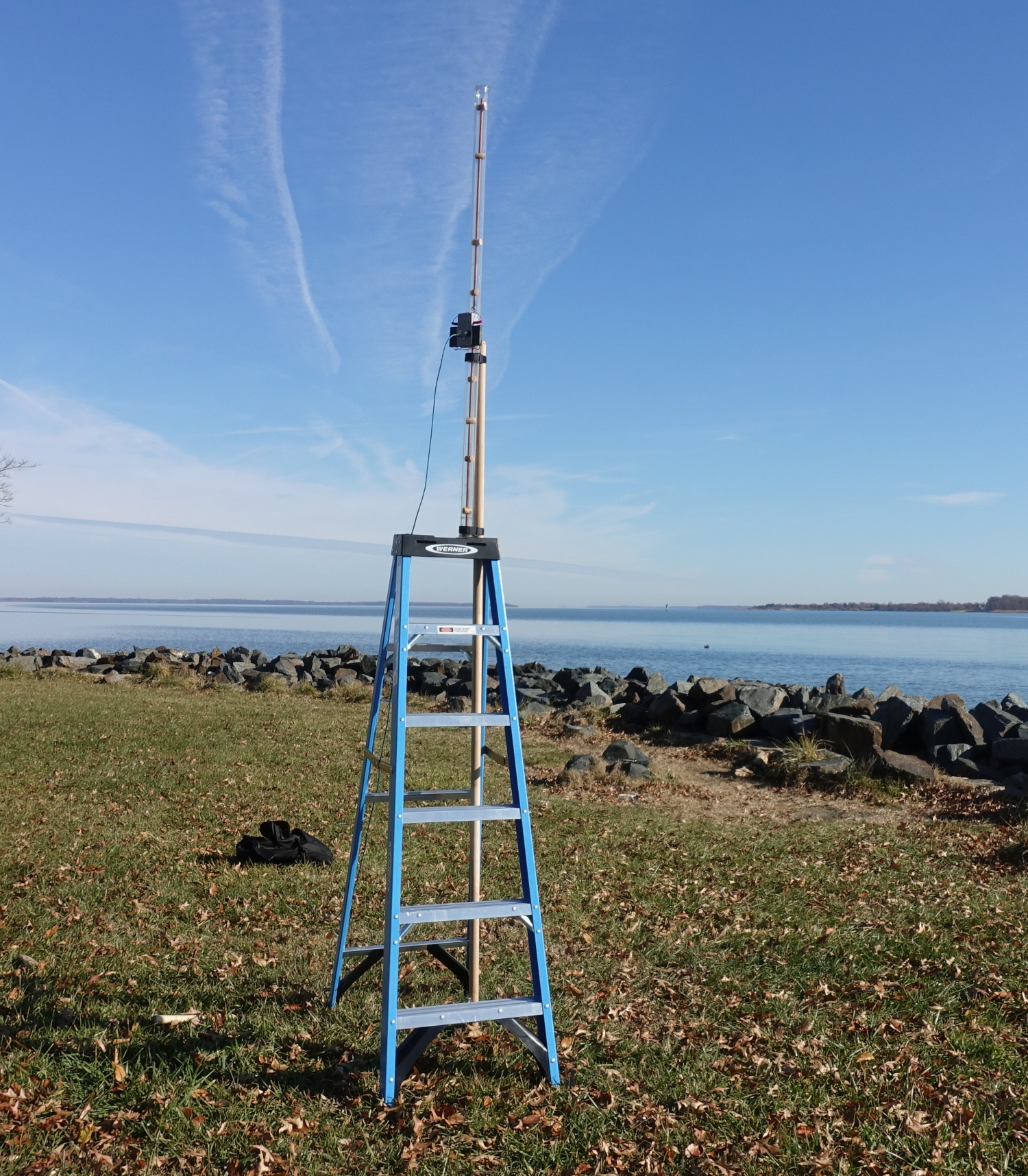
In search of a radio-quiet location, I recently made a recording at the Blackwater National Wildlife Refuge on Maryland's eastern shore:
Dipole Antenna at Blackwater.
While the weather was not perfect (noise from distant lightning) the lack of man-made interference allowed a clean detection of the 2nd through 6th resonances. Here is the plot of the Fourier transform:
Schumann Resonances at Blackwater Refuge.
While the first resonance is buried in noise, it is remarkable that the other resonances (2nd, 3rd, 4th, 5th and 6th at 14.7, 20.2, 27.5, 33.1 and 40.4 Hz) are so strongly visible. (In fact, with careful analysis, the fundamental resonance at 7.8 Hz is present.)
VLF Radio Stations Heard in Turkmenistan
At frequecies between 10kHz and 50kHZ, there are stations worldwide which transmit navigation signals and encoded messages for submarines. While visiting the remains of the 4000 year old civilization at Gonur Depe in Turkmenistan, I took advantage of the lack of radio interference to record the VLF (Very Low Frequency) radio spectrum. Here are the results:
Stations Heard
There are strong stations from all over the globe. The NAA Culter station is in Maine, USA.
The triplet of off-on signals below 15kHz come from different Russian locations, so that timing their arrival can provide the location of the receiver, much like what is done with GPS satellite signals. Very low frequencies penetrate more deeply into sea water, so submarines
can detect them without surfacing.
The Earth's Magnetic Field
The Earth's field is often modeled by a series of spherical harmonics. Here is a J routine that evaluates such an expansion to give the x,y, and z components of the field for any given longitude and latitude:
XYZ.ijs
Relevant Maths
This is a routine to solve for the root of a (maybe nonlinear) equation, using
Brent's method:
brent.ijs.
This is a Runge-Kutta integration routine for ordinary differential equations:
runge_kutta.ijs.
This is an integration routine for stiff systems of differential equations:
stiff.ijs.
These are spline interpolation and integration routines:
splines.ijs.
If we have a fixed "x" grid but many different functions y(x), it may
be useful to precompute a matrix "B" such that (B times y) gives the 2nd
derivatives for the spline fit to y(x). This J routine finds such a matrix:
SpMD.ijs. SpMD assumes a "natural" cubic spline, i.e.,
the first and last 2nd derivatives are set to zero. A more general case is
given by SpMDD.ijs, where you may specify the first
derivative at either or both boundaries. SpMD is useful in constructing
matrix representations for the integral of a function against a known kernel
function, where the integrals of x^n * kernel(x) are analytic. (See the
radiative transfer routines above.)
If we have many data points but they have some associated error, we may want
to fit a cubic spline using a least squares approach. Here is code to make
and evaluate such least squares splines. This is an
example of such a fit: Fit to titanium heat data.
Here is a function for 2-D bicubic interpolation:
bcuint.ijs.
The exponential integral function is used frequently in
radiative transfer calculations:
Ei.ijs.
Here is a better version that works on arrays (it's much faster for typical J applications):
EIn.ijs.
Here are some utilities to manipulate quaternions:
Quaternions.ijs.
(Quaternions are useful, for example,
in rotating coordinates in scattering problems.)
E.g., for fast rotations: qRot.ijs.
These find the coefficients of the Legendre polynomials
and thus find roots and weights for Gaussian quadrature.
LegP_coeff.ijs.
The Associated Legendre polynomials are needed for spherical harmonics.
They may be calculated with Plegendre.ijs.
Given three points on a circle, find the center and radius:
fit_circle.ijs.
You can call LAPACK linear algebraic routines from J.
Here is an example using this to get the roots of a polynomial:
poly_root.ijs.
Bernstein polynomials are used for Bezier curves:
Bezier.ijs.
Here is code for the Incomplete Gamma Function:
GamInc.ijs.