Wavelength calibration involves solving the equation relating wavelength and plate spacing for the slope B and zero-point A:
λ = A + B Zfine
Once A and B are known, this equation yields the value of fine plate spacing (Zfine) necessary to observe the wavelength of interest.
A varies with time (possibly due to temperature changes) and with the parallelism setting. It must be calibrated at the beginning of the run and checked frequently using single, full-field images of rings. B (or dλ/dZ) depends on the coarse plate spacing Zcoarse and the interference order. However, it is stable and has been measured for 3 values of Zcoarse in each filter (see the table below).
The instrument scientist provides values of A and B to the astronomer at the beginning of a run. It is the astronomer's responsibility to track changes in A (due to, e.g., temperature drift).
The table below has links to MMTF arc lamp spectra. These were
taken by scanning the etalon spacing through somewhat more than 1 free
spectral range (FSR): a "data sausage." The spectra are acquired using
a small CCD subraster near the optical axis. This table also lists
suggested lamps for doing wavelength calibration and parallelism
tests, including whether it is internal or external ("Int/Ext") and
good exposure times. The final column gives details about the etalon
properties derived from these spectra, including values for B and FWHM
and approximate Zfine ranges used to achieve a particular
order.
| Filter | ZC | Lamp | Int/Ext | texp | Z0 | dZ | nZ | Spectra | Parameter Table |
|---|---|---|---|---|---|---|---|---|---|
| 5100 | -2 | Ne | Int | 15s | 2800 | 15 | 120 | plot | table |
| +1 | Ne | Int | 15s | 2800 | 15 | 120 | plot | ||
| +3 | Ne | Int | 15s | 1800 | 15 | 120 | plot | ||
| 5300 | -2 | Ne | Int | 15s | 2000 | 15 | 130 | plot | table |
| +1 | Ne | Int | 15s | 2000 | 15 | 130 | plot | ||
| +3 | Ne | Int | 15s | 2400 | 15 | 130 | plot | ||
| 6400 | -2 | Ne | Ext | 1s | 1900 | 15 | 100 | plot | table |
| +1 | Ne | Ext | 1s | 1900 | 15 | 100 | plot | ||
| 3 | Ne | Ext | 1s | 1900 | 15 | 100 | plot | ||
| 6600 | -2 | Ne | Ext | 1s | 2000 | 15 | 110 | plot | table |
| +1 | Ne | Ext | 2s | 2000 | 15 | 110 | plot | ||
| +3 | Ne | Ext | 2s | 2000 | 15 | 110 | plot | ||
| 6800 | -2 | Ne | Ext | 1s | 1700 | 15 | 120 | plot | table |
| +1 | Ne | Ext | 3s | 1400 | 15 | 110 | plot | ||
| +3 | Ne | Ext | 3s | 1500 | 15 | 110 | plot | ||
| 7050 | -2 | Ar | Int | 1s | 1800 | 15 | 100 | plot | table |
| +1 | Ar | Int | 2s | 1800 | 15 | 110 | plot | ||
| +3 | Ar | Int | 1s | 1800 | 15 | 120 | plot | ||
| 8200 | -2 | Kr+Xe | Int | 1s | 1800 | 15 | 110 | plot | table |
| +1 | Kr+Xe | Int | 1s | 1800 | 15 | 120 | plot | ||
| +3 | Kr+Xe | Int | 1s | 1600 | 15 | 120 | plot | ||
| 8650 | -2 | Kr+Xe | Int | 1s | 2100 | 15 | 110 | plot | table |
| +1 | Kr+Xe | Int | 1s | 2100 | 15 | 110 | |||
| +3 | Kr+Xe | Int | 1s | 2100 | 15 | 110 | |||
| 9150 | -2 | Xe | Int | 1s | 1500 | 15 | 120 | plot | table |
| +1 | Xe | Int | 2s | 1600 | 15 | 120 | plot | ||
| +3 | Xe | Int | 2s | 1600 | 15 | 120 | plot |
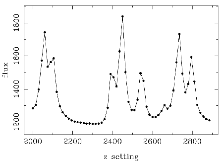
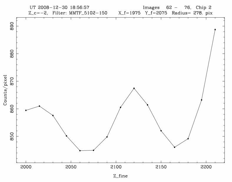
During the afternoon preceding an MMTF run, the instrument scientist provides A and B to the observer for each filter. B comes from the calibration table above, and A from a data sausage (see the figure at right). A reference ring image must also be taken before each data sausage. We describe these procedures below.
- IMPORTANT: This image should be taken immediately before or after a data sausage. The etalon should also be parallelized before any wavelength calibration proceeds.
- Turn on the lamp suggested for the filter of interest (see table above).
- Vary the etalon Zfine and take Snap exposures until a relatively strong emission-line ring appears in the field-of-view. The ring should be isolated from other lines, and its radius should be approximately halfway between the center and edge of the aperture.
- Take a binned image of the emission-line ring, using the exposure time suggested in the table above. To minimize readout time, use the coarsest binning possible while maintaining an unsaturated image (preferably 8 x 8, but finer binning if necessary).
- Give the number of this exposure, as well as the Zfine used, to the observer.
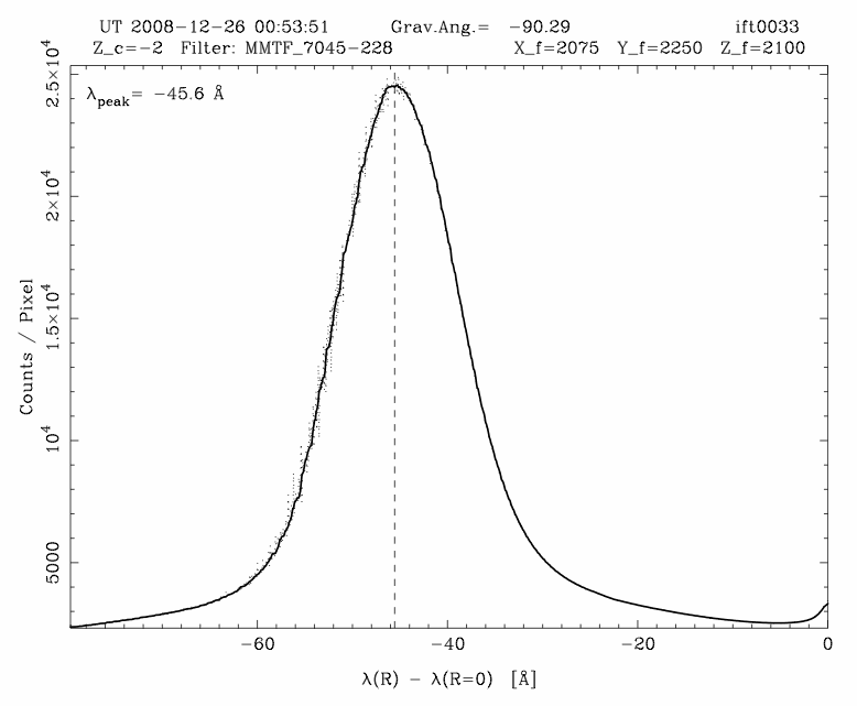
- In a terminal window, check the spectrum by typing the following
(fill in the proper exposure no. and filter central wavelength):
% ring ccd0001 6600
NOTE: If a data sausage for a given configuration (filter and coarse Z) has been acquired recently (since the MMTF was last removed), you may simply use "ringdrift" to find the appropriate change in A. It is safe to assume that B remains the same night-to-night.
- Running a well-sampled data sausage typically takes ~20-30 minutes; this is dominated by CCD readout time.
- Turn on the arc lamp recommended in the table above for the filter of interest.
- Before taking the data sausage, take a reference ring image as described above.
- Turn on CCD subrasters by changing the ExpMode from Full to Subraster. When the subraster menu pops up, load the file defining the MMTF data sausage subrasters: mmtf_sausage.sub in the default path, /Users/imacs/Subrasters/. Click the Load button to load this subraster. REMEMBER: Set the SaveMode to Minimal to minimize readout time. Click Apply. Exit this window by clicking Done.
- Ensure that CCD binning is set to 1x1, and that the exposure time is appropriate for the lamp you are using (the same exposure time as for the reference ring is fine).
- Under the Script menu, click Create. In the pop-up window, select the Scan(seq) Mode. Set Z0 equal to the the lowest Zfine in the reference data sausage spectrum given in the table above. Set dZ (point spacing) to 15, and set nZ (number of points) to the value listed in the above table. The user should try to get 2 full orders, which is typically around nZ=120.
- Save the etalon script.
- To begin the data sausage, click Exec under the Script menu.
- Once the data sausage has finished, type the following in a
terminal window:
% sausage [n0] [n0+nZ] 2
where [n0] and [n0+nZ] are the beginning and ending frame values in the data sausage (leading zeros ignored) and the last number is the IMACS CCD chip. Always use chip 2, which is closest to the optical axis. - Sausage will display a spectrum, which you can compare to the one given in the table. It should have identical shape, but may be shifted. It will then attempt to obtain a calibration line based on your new sausage and pre-loaded data. ALWAYS check the final output plot from sausage, which will have a solid curve, representing the artificial spectrum that has been fit to your data and points representing the data from your sausage. If the curve appears to be a poor fit, calibration may have failed.
Sausage will also display messages to the terminal if it thinks the calibration has failed. Pay attention to these messages. You may need to reparallelize the plates and try again. Make sure that the correct filter is in place and the correct lamp is on. Check to ensure that the z coarse setting used on the etalon is what the output plot says is used. If these are all correct, you may try calibrating the sausage by hand (see below). - If you are satisfied with the fit generated by sausage, the A and B values should be entered into the appropriate fields of the MMTF wavelength calculator (WCALC). Make sure to also write them down in case of a computer failure!
A "data sausage" spectrum, taken by stepping the etalon spacing in small increments through approximately one free spectral range.
During the afternoon preceding your run, the instrument scientist will acquire data sausages/links (see above) and reference ring images to determine the wavelength zero point (A) for each filter you plan to use. He/she will also provide the value of B (see also the table above). It is the observer's responsbility to track changes in A with time. We recommend checking A at least every 30 minutes at the beginning of the night, when the dome temperature changes rapidly.
Changes in A, and hence the values of fine plate spacing necessary to observe the wavelength of interest, are tracked using the MMTF online wavelength calculator (WCALC). To begin, enter the relevant information for your target into WCALC: the value of B provided by the instrument scientist, the wavelength of interest, and the object position with respect to the optical axis (which is approximately at the field center). Next, insert the reference A value into the Aref box, and click the button next to it. This will assign A = Aref and compute the value of Zfine when the reference data was taken.
To update A and Zfine, use the following procedure:
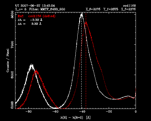
- Take a binned exposure at the same Zfine setting and binning used for the reference image, using the same arc lamp. Let's call the new image ccd1159 and the reference image ccd1156, and assume that we are using the 6400 Å filter.
- In a terminal window, type the following:
% ring ccd1159 6400
% ringdrift 1156 1159
The resulting spectrum is shown at right. - Enter the change in A specified by ringdrift into the ΔA text window in WCALC. Press the "set A = Aref + dA and compute new Z" button.
- Enter the new value of Zfine for the wavelength of interest into the IMACS observing computer.
- Observe!
- This section assumes you have already taken a sausage by following the instructions in the above section.
- type the following in a
terminal window:
% fitsausage [n0] [n0+nZ] 2
where [n0] and [n0+nZ] are the beginning and ending frame values in the data sausage (leading zeros ignored) and the last number is the IMACS CCD chip. Always use chip 2, which is closest to the optical axis. Compare the resulting spectrum to the one given in the table, and make sure it is identical (there may be a small horizontal shift). - Copy the IRAF commands listed by the fitsausage output into an
IRAF terminal window. Using the splot fitting routines, fit Lorentzian profiles to each of the emission lines. For a single line, do the following:
- type 'k' at the continuum level just to the left of the line, and 'l' at the same level to the right
For a doublet, the following procedure will fit two lines simultaneously:- Type 'd' at the continuum level just to the left of the doublet and then 'd' again at the same level to the right.
- Move your mouse to the peak of the first line and type 'l'. Then, move to the second peak and type 'l' again. Finally, type 'q'.
- Type 'a' to fit all centroids, 'a' again to fit all widths, and 'y' to fit background.
The output after the line is fit will contain the centroid position for that line. If you have fit two lines simultaneously, you can view the properties of the next line by typing '+' or the previous line with '-'. To begin fitting a new line, type 'q' and then click your mouse anywhere on the screen to refresh the plot. - Create an ascii file (e.g. params.dat) with a new row for each emission line. The
columns should be: 1 - wavelength, 2 - Z (centroid from splot), 3 -
relative order. The wavelength and relative order can be obtained by
looking at a reference data sausage from the table at the top of
this page (under "Parameter Table"). Run FPSOLVE using the following
syntax:
% fpsolve 1 params.dat
The output of this command will be the A and B parameters for the orders that you sampled. You should be aware of what order you will be operating in for the night, and what the corresponding B term should be. The RMS error in your calibration should be less than an angstrom. If it is too high, try removing one of the lines from your fit (it should be obvious which is contributing most to the error). Alternatively, go back and measure the line centroids more carefully.
Once you are satisfied with the fit, the A and B values should be entered into the appropriate fields of the MMTF wavelength calculator (WCALC). Make sure to also write them down in case of a computer failure!Procedure to acquire a sausage linkNOTE: During normal operation sausage links are unnecessary - careful monitoring of the reference ring is sufficient. However, if the user is lost in wavelength space for some reason, a sausage link is a fast way of re-determining the wavelength zeropoint without performing a full data sausage.
For a sausage link, a bright, isolated (no blends) line should be used, which is as close as possible to the wavelength of interest for the observing run.
- Running a well-sampled sausage link typically takes ~5-10 minutes; this is about equal parts CCD readout time and line fitting.
- Turn on the arc lamp recommended in the table above for the filter of interest.
- Before taking the data sausage, take a reference ring image as described above.
- Turn on CCD subrasters by changing the ExpMode from Full to Subraster. When the subraster menu pops up, load the file defining the MMTF data sausage subrasters: mmtf_sausage.sub in the default path, /Users/imacs/subrasters/. Click the Load button to load this subraster. REMEMBER: Set the SaveMode to Minimal to minimize readout time. Click Apply. Exit this window by clicking Done.
- Ensure that CCD binning is set to 1x1, and that the exposure time is appropriate for the lamp you are using (the same exposure time as for the reference ring is fine).
- Under the Script menu, click Create. In the pop-up window, select the Scan(seq) Mode. Set Z0 so that it is ~50 Zfine units lower than the location of the emission line used in the reference ring. Keep dZ at the default value of 20, and set nZ equal to ~10, or however long it takes to fully sample the emission line.
- Save the etalon script.
- To begin the sausage link, click Exec under the Script menu.
- Once the sausage link has finished, type the following in a
terminal window:
% fitsausage 1 51 2
where the first two numbers are the beginning and ending frame values in the sausage link (leading zeros ignored) and the last number is the IMACS CCD chip. Always use chip 2, which is closest to the optical axis. - Copy the IRAF commands listed by the fitsausage output into an IRAF terminal window. Using the splot fitting routines (e.g., 'k' and 'l' for a single-line fit, or 'd' and 'd' for a multi-line fit), fit a Lorentzian profile to the emission line.
- Insert the wavelength and measured Zfine value of this emission line into the MMTF wavelength calculator (WCALC). Enter the subraster radius output by fitsausage. Enter the appropriate value of B from the table above (for the given filter, Zcoarse value, and interference order corresponding to the emission line that was measured). Click the compute A button, and note the resulting value of A. Give this value to the observer, and copy it to the Aref box in WCALC.
A "sausage link" spectrum, taken by stepping the etalon spacing
in small increments over the range of a single emission line.
